Implementation, Pre-training and Finetuning of BERT
BERT - Bidirectional Encoder Representation with Transformers
It was in 2018 that Google (Devline et al.) published the paper titled “Pre-training of deep bidirectional transformers for language understanding” in which they introduced BERT (Bidirectional Encoder Representation with Transformers) and became a state-of-the-art on many language tasks. In this blog - I decided to find out exactly what happens behind BERT and why it became one of the biggest reasons for the success in language modelling.
Specifically, I’ll be covering the following questions: I am going to explore BERT: what it is? how it works? and how can adapt it for a particular language modelling task?
Table of Contents:
- 1. BERT from scratch
  1.1 Data.................................................
      - 1.1.1 Processing files
      - 1.1.2 Processing the Input
      - 1.1.3 DataLoader for BERT

  1.2 Model
      - 1.2.1 Positional Encoding
      - 1.2.2 Multi-Head Attention
      - 1.2.3 The Encoder
      - 1.2.4 BERT Transformer

  1.3 Training
  1.4 Visualization
- 2. Fine-tuning BERT
  2.1 Dataset.................................................
      - 2.1.1 Downloading SQuAD 2.0 dataset
      - 2.1.2 Load Data
      - 2.1.3 Processing and Tokenization
      - 2.1.4 Correcting Token Positions
      - 2.1.5 Creating DataLoader

  2.2 Model
      - 2.2.1 Loading Pretrained BERT

  2.3 Train

  2.4 Evaluation
      - 2.4.1 Predictions

  2.5 Visualizing
- Discussion
- References
. . .
Reproducibility: After experiencing slow train/infer times, I’ve switched from my usual machine to a more capable machine, and I highly recommend a powerful CPU and GPU in order to complete the training time in resepectable time. This notebook was ran on the following configuration:
- All the cpu-intensive processing is done over
Intel Xeon(R) chipeset. - all the cuda-processing (including training and inference) has been done over
NVIDIA Tesla-P100
!nvidia-smi
+-----------------------------------------------------------------------------+
| NVIDIA-SMI 450.119.04   Driver Version: 450.119.04   CUDA Version: 11.0     |
|-------------------------------+----------------------+----------------------+
| GPU  Name        Persistence-M| Bus-Id        Disp.A | Volatile Uncorr. ECC |
| Fan  Temp  Perf  Pwr:Usage/Cap|         Memory-Usage | GPU-Util  Compute M. |
|                               |                      |               MIG M. |
|===============================+======================+======================|
|   0  Tesla P100-PCIE...  Off  | 00000000:00:04.0 Off |                    0 |
| N/A   36C    P0    27W / 250W |      0MiB / 16280MiB |      0%      Default |
|                               |                      |                  N/A |
+-------------------------------+----------------------+----------------------+

+-----------------------------------------------------------------------------+
| Processes:                                                                  |
|  GPU   GI   CI        PID   Type   Process name                  GPU Memory |
|        ID   ID                                                   Usage      |
|=============================================================================|
|  No running processes found                                                 |
+-----------------------------------------------------------------------------+
import os
import re
import time
import math
import json
import random
import pickle
import string, re
import numpy as np
import pandas as pd
from pathlib import Path
from collections import Counter
from unicodedata import normalize
from IPython.display import display, HTML
from sklearn.model_selection import train_test_split
1. BERT from scratch
To understand the mechanics behind BERT, I start with an implementation of BERT from absolute scratch completely in PyTorch. I do take some necessary assumptions\relaxations along the way in order to make it work, all of which has been documented. My goal with implementing BERT from scratch is nothing but to explore and learn the mechanics of the BERT.
The architecture of BERT has always been quite huge, I just try to implement a lite-version of BERT which is able to learn some representations. I do mention that I’m not focussing on evaluation here as I’ve reserved it for a more capable model described in the next section.
1.1 Data
BERT helps solving one of the biggest challenges in NLP - lack of enough labelled data. As deep learning based NLP models require huge amounts of data in order to perform well, this has been quite an issue. This is where BERT outshines. BERT uses techinques which just the unannotated text to train a general purpose language representation.
Since, my focus in this section is to just plainly design a lite-version of BERT and understand the design choices and its mechanics, I go with a toy dataset. Specifically, I take the English-French translation corpus (can be downloaded from here).
1.1.1 Processing files
-
Function read_data -Read the file in read-only mode and returns a list of sentences in a lin-by-line fashion. -
Function process_data -Normalize text with the UTF-8 so it stays in a human-freiendly readable format. Remove non-information text content like punctuations and other characters. -
Function write_file -Function for writing the text data into a file.
def read_data(filename):
    with open(filename, mode='rt') as f:
        text = f.read()

    lines = text.strip().split('\n')
    data = [line.split('\t') for line in lines]
    return data

def process_data(data):
    cleaned = []

    re_chars = re.compile('[^%s]' % re.escape(string.printable))
    table = str.maketrans('','',string.punctuation)
    for lines in data:
        clean_text = []
        for text in lines:
            text = normalize('NFD', text).encode('ascii', 'ignore')
            text = text.decode('UTF-8').split()
            text = [w.lower() for w in text]
            text = [w.translate(table) for w in text]
            text = [re_chars.sub('', w) for w in text]
            text = [w for w in text if w.isalpha()]
            clean_text.append(' '.join(text))
        cleaned.append(clean_text)
    return np.array(cleaned)

def write_file(filename, text):
    with open(filename, 'w') as f:
        for line in text[:,0]:
            f.write(line)
            f.write("\n")
RAW_FILENAME = '../fra.txt'
PROCESSED_FILENAME = "eng-corpus.txt"

data = read_data(RAW_FILENAME)
text = process_data(data)

np.random.seed(10)
np.random.shuffle(text)
write_file(filename=PROCESSED_FILENAME, text=text)

dataset = {'English': [line for line in text[:,0]]}
df = pd.DataFrame(dataset, columns=["English"])

df['eng_len'] = df['English'].str.count(' ') + 1
display(HTML(df[:30].to_html()))
| English | eng_len | |
|---|---|---|
| 0 | put it in the top dresser drawer | 7 |
| 1 | im so happy to hear that | 6 |
| 2 | whatre you all dressed up for | 6 |
| 3 | i wasnt interested in the job | 6 |
| 4 | is there a mall near here | 6 |
| 5 | are you still studying french | 5 |
| 6 | write to him right away | 5 |
| 7 | did i ask your opinion | 5 |
| 8 | i feel like ive known you forever | 7 |
| 9 | ill just get you started | 5 |
| 10 | im glad its over | 4 |
| 11 | sony is a brand known around the world | 8 |
| 12 | i know this district | 4 |
| 13 | how many years did it take to build the pyramids | 10 |
| 14 | we got stuck in traffic | 5 |
| 15 | it seemed like a good idea | 6 |
| 16 | we moved into this house last month but we still havent settled down | 13 |
| 17 | what movie did you see | 5 |
| 18 | my father doesnt drink so much sake | 7 |
| 19 | i was abducted by aliens | 5 |
| 20 | how soon do you need it | 6 |
| 21 | theyre bad | 2 |
| 22 | this kind of work makes me hungry | 7 |
| 23 | some tv programs are interesting and others are not | 9 |
| 24 | none of us can see them | 6 |
| 25 | online banking is very convenient | 5 |
| 26 | you alone can do it but you cant do it alone | 11 |
| 27 | my sister is pretty | 4 |
| 28 | i must find out who is behind this | 8 |
| 29 | id like to confirm my reservation for the | 8 |
1.1.2 Processing the Input
We now have the cleaned version of data. Since, transformer models like BERT work at the sentence level with decomposed words, I can directly load the stored file. Like any language model, the natural step after cleaning the data is generating the vocabulary.
Function generate_vocab - The function to generate the vobaulary and store it as vocab.txt which will be used later.
N_VOCAB = 20000

def generate_vocab(filename, n_vocab):
    sentences = open(filename).read().lower().split('\n')
    sentences = [s.split(' ') for s in sentences]
    sentences = [[w for w in s if len(w)] for s in sentences]

    print('Creating vocab...')
    VOCAB_FILENAME = 'vocab.txt'

    if not os.path.exists(VOCAB_FILENAME):
        words = [w for s in sentences for w in s]
        vocab = Counter(words).most_common(n_vocab)
        vocab = [w[0] for w in vocab]
        open(VOCAB_FILENAME, 'w+').write('\n'.join(vocab))

    else:
        vocab = open(VOCAB_FILENAME).read().split('\n')
    print("Vocabulary build done!")
    return sentences, vocab
sentences, vocab = generate_vocab(filename=PROCESSED_FILENAME, n_vocab=N_VOCAB)
Creating vocab...
Vocabulary build done!
import torch
import torch.nn as nn
import torch.optim as optim
import torch.nn.functional as F
from torch.utils.data import Dataset
1.1.3 DataLoader for BERT
One of the best things about training BERT is that we dont need labels and only need sentences that we processed earlier.
While going through the paper, what I’ve relized is that BERT doesn’t actually bring a new architecture, rather It just brings idea of masking which was new for the transformers.
Masking: Consider a sentence of 10 words, in this case, 30% masking would mean it’ll remove 3 random words and it’ll be upto the model to predict those words based on the rest of the words in the sentence. The authors of Devlin et al. refers to this idea as the masked language model.
Next Sentence prediction: BERT training process also incorporates next sentence prediction. During training the model gets as input pairs of sentences and it learns to predict if the second sentence is the next sentence in the original text as well.
-
class SentenceDataset -Function for processing the input-output pairs based on the training techniques defined for the BERT model. First, all the sentences, the vocabulary and the sequence length (for batch) is loaded. I define some tags which has the following roles:-
<ignore>:Tag which informs the model to ignore predicting non-masked words as we are only interested in the loss of the masked words. -
<mask>:The tag responsible for masking the word embeddings. -
<sep>:The tag for seperating the two sentences (For Next Sentence Prediction) -
<cls>:The tag added to the begining of sentence.
-
How I am making the “masked language model” work is that, if a word in a sentence is set to mask, then input should have token of
Function get_batch -Function providing batch-wise data iterator.
The data is set to have a batch-size of 128 and a sequence length of 20
class SentencesDataset(Dataset):
    def __init__(self, sentences, vocab, seq_len):
        dataset = self
        dataset.sentences = sentences
        dataset.vocab = vocab + ['<ignore>', '<unk>', '<mask>', '<sep>', '<cls>']
        dataset.vocab = {e:i for i, e in enumerate(dataset.vocab)}
        dataset.rvocab = {v:k for k,v in dataset.vocab.items()}
        dataset.seq_len = seq_len

        dataset.IGNORE_IDX = dataset.vocab['<ignore>']
        dataset.OUT_OF_VOCAB_IDX = dataset.vocab['<unk>']
        dataset.MASK_IDX = dataset.vocab['<mask>']
        dataset.SEP_IDX = dataset.vocab['<sep>']
        dataset.CLS_IDX = dataset.vocab['<cls>']

    def __getitem__(self, index, p_random_mask=0.15, nsp=False):
        dataset = self
        s = []

        while len(s) < dataset.seq_len:
            s.extend(dataset.get_sentence_idx(index % len(dataset)))
            index += 1

        s = s[:dataset.seq_len]
        [s.append(dataset.IGNORE_IDX) for i in range(dataset.seq_len - len(s))] #PAD ok

        joint_s = None
        if nsp:
            current_s = dataset.CLS_IDX + s
            next_s = dataset.get_sentence_idx(index % len(dataset)
            next_s = next_s[:seqlen]
            joint_s = current_s + dataset.SEP_IDX + next_s

        s = [(dataset.MASK_IDX, w) if random.random() < p_random_mask else (w, dataset.IGNORE_IDX) for w in s]
        if nsp:
            return {'input': torch.Tensor([w[0] for w in joint_s]).long(), 'target': torch.Tensor([w[1] for w in joint_s]).long()}

        return {'input': torch.Tensor([w[0] for w in s]).long(), 'target': torch.Tensor([w[1] for w in s]).long()}

    def __len__(self):
        return len(self.sentences)

    def get_sentence_idx(self, index):
        dataset = self
        s = dataset.sentences[index]
        s = [dataset.vocab[w] if w in dataset.vocab else dataset.OUT_OF_VOCAB_IDX for w in s]
        return s


def get_batch(loader, loader_iter):
    try:
        batch = next(loader_iter)
    except StopIteration:
        loader_iter = iter(loader)
        batch = next(loader_iter)
    return batch, loader_iter
BATCH_SIZE = 128
SEQ_LEN = 20
n_workers = 12

dataset = SentencesDataset(sentences, vocab, seq_len=SEQ_LEN)
kwargs = {'num_workers':n_workers, 'shuffle':True,  'drop_last':True, 'pin_memory':True, 'batch_size':BATCH_SIZE}
data_loader = torch.utils.data.DataLoader(dataset, **kwargs)
1.2 Model
At the core BERT still uses a transformer. The novelty that BERT brings is in the idea of bidirectionally training which is new to the transformer. Instead of predicting the next word, it tried to mask words in a sentence and predict them. At an architecture level, the core remains almost the same as that of a Transformer except for some tweaks to make the new tranining strategy work.
1.2.1 Positional Encoding
BERT relies on a Transformer-based mechanism. For this to work, the first component it needs is the input with some extra metadata, i.e, Positional embeddings. BERT requires a seperate implementation of Positional embedding because the basic Transformer can’t process positions in a sequence by itself.
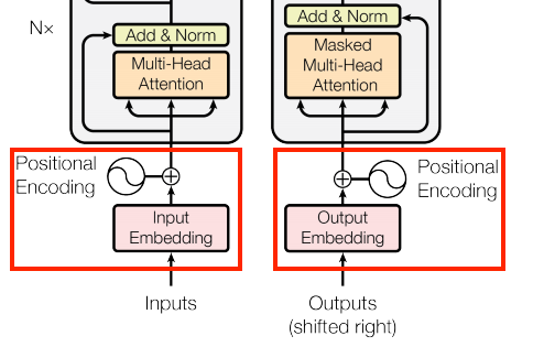
Figure 1. The Position encoding step highlighted in red
I did notice that the Positional embedding/encoding has the same dimension as that of Word embedding (defined later). This can be seen from Figure 1. as it is added with the embedding before passing into the multi-head attention modules.
While I do wonder if directly using the position value would work or not, since it’s quite straightforward way to pass the positional information of the tokens. I’ll stick with the standard way of defining positional embedding, i.e, combination of sinusoidal functions to encode position of token in the sequence.
Class PositionalEmbeddingInitialized the positional encodings and could be accessed with justforwardfunction.
class PositionalEmbedding(nn.Module):
    def __init__(self, d_model, max_seq_len = 80):
        super().__init__()
        self.d_model = d_model
        pe = torch.zeros(max_seq_len, d_model)
        pe.requires_grad = False
        for pos in range(max_seq_len):
            for i in range(0, d_model, 2):
                pe[pos, i] = math.sin(pos / (10000 ** ((2 * i)/d_model)))
                pe[pos, i + 1] = math.cos(pos / (10000 ** ((2 * (i + 1))/d_model)))
        pe = pe.unsqueeze(0)
        self.register_buffer('pe', pe)

    def forward(self, x):
        return self.pe[:,:x.size(1)]
While it never occured to me, when trying implement and make the Transformer work, what I realized is that Transformer is in short, an encoder architecture, atleast in the case of BERT.
1.2.2 Multi-Head Attention
Now, One of the core components that a Transformer uses is a Multi-Head attention. It uses the basic mechanism of attention and replicates it $h$ times. The idea of attention is to turn the input embeddings (Q, K, V) into three word embeddings. Multi-Head just computes this attention map $h$ times each with different weight matrices and then concatenates all the results together.
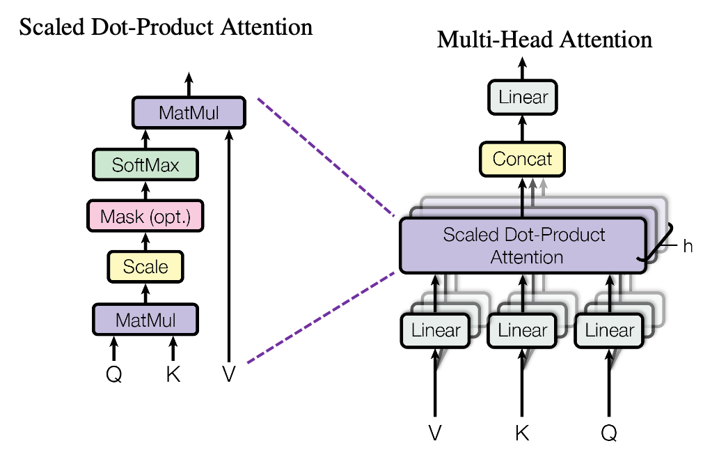 Each of these parallel computations of attention is called as a head, hence the name Multi-Head attention. The three encodings are as follows:
- Query (Q): Main representation of the word
- Key (K): Representions of words being compared with the main word
-
Value (V): Representaion used to produce final embedding of the main word
Function attention -Implements the basic attention mechanism. Mathematically, it can be represented as:
Class MultiHeadAttention -Implements the above described Mutli-Head attention mechanism. Mathematically, it can be represented as:
def attention(q, k, v, mask = None, dropout = None):
    scores = q.matmul(k.transpose(-2, -1))
    scores /= math.sqrt(q.shape[-1])

    scores = scores if mask is None else scores.masked_fill(mask == 0, -1e3)

    scores = F.softmax(scores, dim = -1)
    scores = dropout(scores) if dropout is not None else scores
    output = scores.matmul(v)
    return output


class MultiHeadAttention(nn.Module):
    def __init__(self, n_heads, out_dim, dropout=0.1):
        super().__init__()

        self.linear = nn.Linear(out_dim, out_dim*3)
        self.n_heads = n_heads
        self.out_dim = out_dim
        self.out_dim_per_head = out_dim // n_heads
        self.out = nn.Linear(out_dim, out_dim)
        self.dropout = nn.Dropout(dropout)

    def split_heads(self, t):
        return t.reshape(t.shape[0], -1, self.n_heads, self.out_dim_per_head)

    def forward(self, x, y=None, mask=None):

        y = x if y is None else y
        qkv = self.linear(x)
        q = qkv[:, :, :self.out_dim]
        k = qkv[:, :, self.out_dim:self.out_dim*2]
        v = qkv[:, :, self.out_dim*2:]

        q, k, v = [self.split_heads(t) for t in (q,k,v)]
        q, k, v = [t.transpose(1,2) for t in (q,k,v)]

        scores = attention(q, k, v, mask, self.dropout)
        scores = scores.transpose(1,2).contiguous().view(scores.shape[0], -1, self.out_dim)
        out = self.out(scores)

        return out
1.2.3 The Encoder
Now that we have the attention-based components ready, we can finally develop the whole encoder of the Transformer.
-
Class FeedForward -Implements the Feed forward fully-connected layer with dropouts. -
Class EncoderLayer -Implements the encoder, calling the already defined Multi-Head attention and Feed-forward layers.
One interesting thing to note here is that, the connections are residual meaning, it doesn’t completely changes the raw embeddings but rather adds over what has been already computed. This actually should lead to an enhancing of the existing representations as compared to completely generating a new one. The encoder also incorporates Layer normalization and will thus lead to an effiency in training.
class FeedForward(nn.Module):
    def __init__(self, inp_dim, inner_dim, dropout=0.1):
        super().__init__()
        self.linear1 = nn.Linear(inp_dim, inner_dim)
        self.linear2 = nn.Linear(inner_dim, inp_dim)
        self.dropout = nn.Dropout(dropout)

    def forward(self, x):
        return self.linear2(self.dropout(F.relu(self.linear1(x))))

class EncoderLayer(nn.Module):
    def __init__(self, n_heads, inner_transformer_size, inner_ff_size, dropout=0.1):
        super().__init__()
        self.mha = MultiHeadAttention(n_heads, inner_transformer_size, dropout)
        self.ff = FeedForward(inner_transformer_size, inner_ff_size, dropout)
        self.norm1 = nn.LayerNorm(inner_transformer_size)
        self.norm2 = nn.LayerNorm(inner_transformer_size)
        self.dropout1 = nn.Dropout(dropout)
        self.dropout2 = nn.Dropout(dropout)

    def forward(self, x, mask=None):
        x2 = self.norm1(x)
        x = x + self.dropout1(self.mha(x2, mask=mask))
        x2 = self.norm2(x)
        x = x + self.dropout2(self.ff(x2))
        return x
1.2.4 BERT Transformer
Finally, we combine all the defined modules to construct the transformer.
Do note that my implementation of BERT consists of just a set of encoders. We can always add some layers on top of BERT to tune it for a particular task but, BERT in its raw format, I have made it as a barebones for any language related tasks.
Class BERT -Implements BERT model by calling all the modules which we defined above. Do note here that I’ve set the embedding size to be 128 which is lower as compared the 768 in the original implementation of BERT by Devlin et al.. Since, my aim with this implementation was just to be able to re-create the BERT model, I’m sticking with a smaller model to keep it efficient.
I’ve set the model to have 8 number of attention heads and a dropout rate of 0.1.
class BERT(nn.Module):
    def __init__(self, n_code, n_heads, embed_size, inner_ff_size, n_embeddings, seq_len, dropout=.1):
        super().__init__()

        self.embeddings = nn.Embedding(n_embeddings, embed_size)
        self.pe = PositionalEmbedding(embed_size, seq_len)

        encoders = []
        for i in range(n_code):
            encoders += [EncoderLayer(n_heads, embed_size, inner_ff_size, dropout)]
        self.encoders = nn.ModuleList(encoders)

        self.norm = nn.LayerNorm(embed_size)
        self.linear = nn.Linear(embed_size, n_embeddings, bias=False)


    def forward(self, x):
        x = self.embeddings(x)
        x = x + self.pe(x)
        for encoder in self.encoders:
            x = encoder(x)
        x = self.norm(x)
        x = self.linear(x)
        return x
EMBED_SIZE = 128
ENC_SIZE = EMBED_SIZE * 4
N_HEADS = 8
N_CODE = 8
DROPOUT = 0.1

model = BERT(n_code=N_CODE, n_heads=N_HEADS, embed_size=EMBED_SIZE, inner_ff_size=ENC_SIZE,
                    n_embeddings=len(dataset.vocab), seq_len=SEQ_LEN, dropout=DROPOUT)

optimizer = optim.Adam(model.parameters(), lr=2e-3, weight_decay=1e-4, betas=(.9,.999))
loss_model = nn.CrossEntropyLoss(ignore_index=dataset.IGNORE_IDX)

model = model.cuda()
print("Model Architecture:\n")
print(model)


print(f'\nNo. of trainable parameters: {sum(p.numel() for p in model.parameters() if p.requires_grad):,}')
Model Architecture:

BERT(
  (embeddings): Embedding(15568, 128)
  (pe): PositionalEmbedding()
  (encoders): ModuleList(
    (0): EncoderLayer(
      (mha): MultiHeadAttention(
        (linear): Linear(in_features=128, out_features=384, bias=True)
        (out): Linear(in_features=128, out_features=128, bias=True)
        (dropout): Dropout(p=0.1, inplace=False)
      )
      (ff): FeedForward(
        (linear1): Linear(in_features=128, out_features=512, bias=True)
        (linear2): Linear(in_features=512, out_features=128, bias=True)
        (dropout): Dropout(p=0.1, inplace=False)
      )
      (norm1): LayerNorm((128,), eps=1e-05, elementwise_affine=True)
      (norm2): LayerNorm((128,), eps=1e-05, elementwise_affine=True)
      (dropout1): Dropout(p=0.1, inplace=False)
      (dropout2): Dropout(p=0.1, inplace=False)
    )
    (1): EncoderLayer(
      (mha): MultiHeadAttention(
        (linear): Linear(in_features=128, out_features=384, bias=True)
        (out): Linear(in_features=128, out_features=128, bias=True)
        (dropout): Dropout(p=0.1, inplace=False)
      )
      (ff): FeedForward(
        (linear1): Linear(in_features=128, out_features=512, bias=True)
        (linear2): Linear(in_features=512, out_features=128, bias=True)
        (dropout): Dropout(p=0.1, inplace=False)
      )
      (norm1): LayerNorm((128,), eps=1e-05, elementwise_affine=True)
      (norm2): LayerNorm((128,), eps=1e-05, elementwise_affine=True)
      (dropout1): Dropout(p=0.1, inplace=False)
      (dropout2): Dropout(p=0.1, inplace=False)
    )
    (2): EncoderLayer(
      (mha): MultiHeadAttention(
        (linear): Linear(in_features=128, out_features=384, bias=True)
        (out): Linear(in_features=128, out_features=128, bias=True)
        (dropout): Dropout(p=0.1, inplace=False)
      )
      (ff): FeedForward(
        (linear1): Linear(in_features=128, out_features=512, bias=True)
        (linear2): Linear(in_features=512, out_features=128, bias=True)
        (dropout): Dropout(p=0.1, inplace=False)
      )
      (norm1): LayerNorm((128,), eps=1e-05, elementwise_affine=True)
      (norm2): LayerNorm((128,), eps=1e-05, elementwise_affine=True)
      (dropout1): Dropout(p=0.1, inplace=False)
      (dropout2): Dropout(p=0.1, inplace=False)
    )
    (3): EncoderLayer(
      (mha): MultiHeadAttention(
        (linear): Linear(in_features=128, out_features=384, bias=True)
        (out): Linear(in_features=128, out_features=128, bias=True)
        (dropout): Dropout(p=0.1, inplace=False)
      )
      (ff): FeedForward(
        (linear1): Linear(in_features=128, out_features=512, bias=True)
        (linear2): Linear(in_features=512, out_features=128, bias=True)
        (dropout): Dropout(p=0.1, inplace=False)
      )
      (norm1): LayerNorm((128,), eps=1e-05, elementwise_affine=True)
      (norm2): LayerNorm((128,), eps=1e-05, elementwise_affine=True)
      (dropout1): Dropout(p=0.1, inplace=False)
      (dropout2): Dropout(p=0.1, inplace=False)
    )
    (4): EncoderLayer(
      (mha): MultiHeadAttention(
        (linear): Linear(in_features=128, out_features=384, bias=True)
        (out): Linear(in_features=128, out_features=128, bias=True)
        (dropout): Dropout(p=0.1, inplace=False)
      )
      (ff): FeedForward(
        (linear1): Linear(in_features=128, out_features=512, bias=True)
        (linear2): Linear(in_features=512, out_features=128, bias=True)
        (dropout): Dropout(p=0.1, inplace=False)
      )
      (norm1): LayerNorm((128,), eps=1e-05, elementwise_affine=True)
      (norm2): LayerNorm((128,), eps=1e-05, elementwise_affine=True)
      (dropout1): Dropout(p=0.1, inplace=False)
      (dropout2): Dropout(p=0.1, inplace=False)
    )
    (5): EncoderLayer(
      (mha): MultiHeadAttention(
        (linear): Linear(in_features=128, out_features=384, bias=True)
        (out): Linear(in_features=128, out_features=128, bias=True)
        (dropout): Dropout(p=0.1, inplace=False)
      )
      (ff): FeedForward(
        (linear1): Linear(in_features=128, out_features=512, bias=True)
        (linear2): Linear(in_features=512, out_features=128, bias=True)
        (dropout): Dropout(p=0.1, inplace=False)
      )
      (norm1): LayerNorm((128,), eps=1e-05, elementwise_affine=True)
      (norm2): LayerNorm((128,), eps=1e-05, elementwise_affine=True)
      (dropout1): Dropout(p=0.1, inplace=False)
      (dropout2): Dropout(p=0.1, inplace=False)
    )
    (6): EncoderLayer(
      (mha): MultiHeadAttention(
        (linear): Linear(in_features=128, out_features=384, bias=True)
        (out): Linear(in_features=128, out_features=128, bias=True)
        (dropout): Dropout(p=0.1, inplace=False)
      )
      (ff): FeedForward(
        (linear1): Linear(in_features=128, out_features=512, bias=True)
        (linear2): Linear(in_features=512, out_features=128, bias=True)
        (dropout): Dropout(p=0.1, inplace=False)
      )
      (norm1): LayerNorm((128,), eps=1e-05, elementwise_affine=True)
      (norm2): LayerNorm((128,), eps=1e-05, elementwise_affine=True)
      (dropout1): Dropout(p=0.1, inplace=False)
      (dropout2): Dropout(p=0.1, inplace=False)
    )
    (7): EncoderLayer(
      (mha): MultiHeadAttention(
        (linear): Linear(in_features=128, out_features=384, bias=True)
        (out): Linear(in_features=128, out_features=128, bias=True)
        (dropout): Dropout(p=0.1, inplace=False)
      )
      (ff): FeedForward(
        (linear1): Linear(in_features=128, out_features=512, bias=True)
        (linear2): Linear(in_features=512, out_features=128, bias=True)
        (dropout): Dropout(p=0.1, inplace=False)
      )
      (norm1): LayerNorm((128,), eps=1e-05, elementwise_affine=True)
      (norm2): LayerNorm((128,), eps=1e-05, elementwise_affine=True)
      (dropout1): Dropout(p=0.1, inplace=False)
      (dropout2): Dropout(p=0.1, inplace=False)
    )
  )
  (norm): LayerNorm((128,), eps=1e-05, elementwise_affine=True)
  (linear): Linear(in_features=128, out_features=15568, bias=False)
)

No. of trainable parameters: 27,859,200
As can be seen from above, even though I went with a much lower embedding dimension, even then the model ends up having about ~ 27.8 million paratmeters, which is still quite heavy especially if the training is considered from absolute scratch
1.3 Training
Now we have all the necessary implementation ready, we can start training of the model.
Function evaluate:The function that handles the actual training.
The model is trained for 20 epochs.
BATCH_PRINT = 2
EPOCHS = 10

def train(mdoel, epochs, print_each):
    print('Begining Training...')
    model.train()
    batch_iter = iter(data_loader)

    START = time.time()
    losses = []
    for each_epoch in range(epochs):
        for each_batch in range(1000):
            batch, batch_iter = get_batch(data_loader, batch_iter)

            masked_input = batch['input']
            masked_target = batch['target']

            masked_input = masked_input.cuda(non_blocking=True)
            masked_target = masked_target.cuda(non_blocking=True)
            output = model(masked_input)

            output_v = output.view(-1,output.shape[-1])
            target_v = masked_target.view(-1,1).squeeze()
            loss = loss_model(output_v, target_v)

            loss.backward()
            losses.append(loss)
            optimizer.step()
            optimizer.zero_grad()

        if each_epoch % print_each == 0:
            print('Iteration:', each_epoch,  ' | loss', np.round(loss.item(),2),
                  ' | Time taken ', np.round((time.time() - START)/60, 2), 'mins.')

    return model, losses

start = time.time()
model, losses = train(model, epochs=EPOCHS, print_each=BATCH_PRINT)
print(f"\nTotal time taken: {time.time()-start/60:.2f} mins")
Begining Training...
Iteration: 0 | loss: 5.26 | Time taken 16.6 mins.
Iteration: 1 | loss: 4.49 | Time taken 16.6 mins.
Iteration: 2 | loss: 3.71 | Time taken 16.6 mins.
Iteration: 3 | loss: 3.14 | Time taken 16.5 mins.
Iteration: 4 | loss: 2.69 | Time taken 16.5 mins.
Iteration: 5 | loss: 2.05 | Time taken 16.5 mins.
Iteration: 6 | loss: 1.87 | Time taken 16.6 mins.
Iteration: 7 | loss: 1.63 | Time taken 16.6 mins.
Iteration: 8 | loss: 1.57 | Time taken 16.5 mins.
Iteration: 9 | loss: 1.49 | Time taken 16.6 mins.

Total time taken: 165.60 mins
import matplotlib.pyplot as plt
import pandas as pd

def plot_losses(losses, epochs=10):
    df = pd.DataFrame(losses, columns =['Loss'])

    df['Epochs'] = list(range(1,epochs+1))

    with plt.style.context('seaborn'):
        df.plot(x='Epochs',y=['Loss'], figsize=(14,10))


plot_losses(losses, epochs=10)

As can be seen from the above results, training has been quite converging indicating that the model was able to learn some basic word representations.
print('Saving top embeddings...')
top_k = 3000
np.savetxt('values.tsv', np.round(model.embeddings.weight.detach().cpu().numpy()[0:top_k], 2), delimiter='\t', fmt='%1.2f')
topk_words = [dataset.rvocab[i] for i in range(top_k)]
open('names.tsv', 'w+').write('\n'.join(topk_words) )
Saving top embeddings...


21190
1.5 Visualization
Next I try to visualize embeddings of the top-k words where k = 500.
Function plotTSNE -In order to plot the embeddings, I run t-SNE (T-distributed Stochastic Neighbor Embedding) algorithm which is a dimensionality reduction tenchnique used to visualize high-dimensional data. After doing dimensionality reduction to just 2 components, I plot them in a 2-D space.
!pip install plotly==4.0.0
huggingface/tokenizers: The current process just got forked, after parallelism has already been used. Disabling parallelism to avoid deadlocks...
To disable this warning, you can either:
	- Avoid using `tokenizers` before the fork if possible
	- Explicitly set the environment variable TOKENIZERS_PARALLELISM=(true | false)
Collecting plotly==4.0.0
  Downloading plotly-4.0.0-py2.py3-none-any.whl (6.8 MB)
     |████████████████████████████████| 6.8 MB 28.4 MB/s
Collecting retrying>=1.3.3
  Downloading retrying-1.3.3.tar.gz (10 kB)
  Preparing metadata (setup.py) ...
import pandas as pd

import plotly
import plotly.express as px
from plotly.offline import init_notebook_mode, iplot

import matplotlib.pyplot as plt
from sklearn.manifold import TSNE

top_k = 500
values = pd.read_csv('../try1/values.tsv', sep='\t', header=None)
with open('../try1/names.tsv', 'r') as f:
    lines = [line.rstrip() for line in f]
# plt.style.library['ggplot']

def plotTSNE(top_k):
    words = lines[:500]
    model = TSNE(n_components=2, perplexity=5, init='pca', method='exact', n_iter=5000)
    X = model.fit_transform(values[:500])
    plt.figure(figsize=(18, 18))
    for i in range(len(X)):
        plt.text(X[i, 0], X[i, 1], words[i], bbox=dict(facecolor='red', alpha=0.05))
    plt.xlim((np.min(X[:, 0]), np.max(X[:, 0])))
    plt.ylim((np.min(X[:, 1]), np.max(X[:, 1])))
    plt.show()

with plt.style.context('seaborn'):
    plotTSNE(top_k=top_k)
The default learning rate in TSNE will change from 200.0 to 'auto' in 1.2.

The PCA initialization in TSNE will change to have the standard deviation of PC1 equal to 1e-4 in 1.2. This will ensure better convergence.
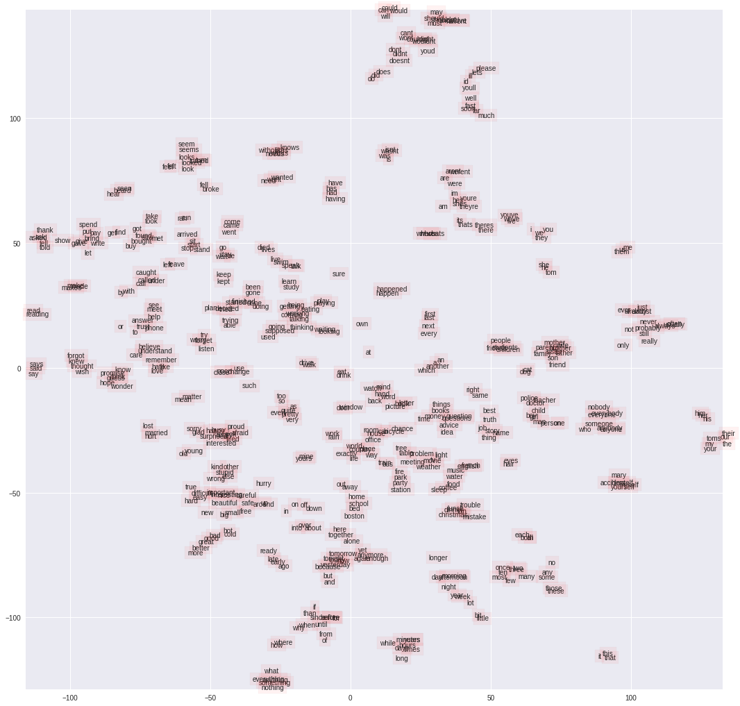
We can see that many words with identical semantics are grouped together. Some of the very easy to observe groups are 1. (day, year, week, month), 2. (do, don’t, does, doesn’t), 3. (mother, father, daughter…) etc. Interestingly Boston has an embedding paired with colleges and I think that’s indicating the information that Boston is famous of the best schools and this ingormation might’ve been referred to in text as well.
.
.
2 Fine-tuning BERT
In the next section, I take one of the state-of-the-art pretrained versions of BERT, and explore how we could fine-tune a pretrained model and do inference\analysis on task-specific datasets.
Spefically, I consider the task of question of Question-Answering and use the one of the highly cited datasets - SQuAD-v2. I’ll try to explore how good we can fine-tune it and analyse its results on unseen text. I’ve also tried to validate the models by visualizing the attention weights during a particlar instance of inference. Finally, I generate predictions on SQuAD-v2 dev version (validation set) and make it avaiable for Reza Akbarian Bafghi for evaluation and comparison on its results with the baseline.
Transformer library
I’ll be using the python-package transformers. This package is open-source and contains the implementation of different varities of pretrained models. Importantly, it also contains many functionalities which makes it easier to fine-tune a Transformer-based model. Lastly it provides some hidden perks for visualization which could be quite powerful in analysing the model (See Visualization section below)
!pip install transformers

from transformers import AutoTokenizer, AdamW, BertForQuestionAnswering
2.1 Dataset
The Stanford Question Answering Dataset (SQuAD) is one of the most common benchmarks in NLP. It consists of more than 1000,000 set of Wikipedia articles, where the answer to every question is a segment of text, or span, from the corresponding reading passage. I specifically use SQuAD-v2 which is an updated version of squad. It adds negative samples into the data, where a negative sample refers to simply not having an answer.
The reason that I use SQuAD-v2 is that a model fine-tuned in this dataset, not only has to answer questions when possible, but also determine when there is no answer supported by the paragraph and should abstain from answering.
2.1.1 Downloading SQuAD 2.0 dataset
The SQuAD-v2 dataset is publicly available and could be downloaded from Rajpurkar’s site (developer)
!mkdir squad
!wget https://rajpurkar.github.io/SQuAD-explorer/dataset/train-v2.0.json -O squad/train-v2.0.json
!wget https://rajpurkar.github.io/SQuAD-explorer/dataset/dev-v2.0.json -O squad/dev-v2.0.json
--2022-02-22 21:13:35--  https://rajpurkar.github.io/SQuAD-explorer/dataset/train-v2.0.json
Resolving rajpurkar.github.io (rajpurkar.github.io)... 185.199.109.153, 185.199.108.153, 185.199.111.153, ...
Connecting to rajpurkar.github.io (rajpurkar.github.io)|185.199.109.153|:443... connected.
HTTP request sent, awaiting response... 200 OK
Length: 42123633 (40M) [application/json]
Saving to: ‘squad/train-v2.0.json’

squad/train-v2.0.js 100%[===================>]  40.17M   111MB/s    in 0.4s

2022-02-22 21:13:36 (111 MB/s) - ‘squad/train-v2.0.json’ saved [42123633/42123633]

--2022-02-22 21:13:36--  https://rajpurkar.github.io/SQuAD-explorer/dataset/dev-v2.0.json
Resolving rajpurkar.github.io (rajpurkar.github.io)... 185.199.110.153, 185.199.111.153, 185.199.108.153, ...
Connecting to rajpurkar.github.io (rajpurkar.github.io)|185.199.110.153|:443... connected.
HTTP request sent, awaiting response... 200 OK
Length: 4370528 (4.2M) [application/json]
Saving to: ‘squad/dev-v2.0.json’

squad/dev-v2.0.json 100%[===================>]   4.17M  --.-KB/s    in 0.04s

2022-02-22 21:13:36 (103 MB/s) - ‘squad/dev-v2.0.json’ saved [4370528/4370528]
2.1.2 Load Data
Function load_data -I read and store the texts, queries and answers from the train and validation set of SQuAD data.
TRAIN_DIR = Path('squad/train-v2.0.json')
DEV_DIR = Path('squad/dev-v2.0.json')

def load_data(path, data_type=None):

    print(f"Processing {data_type}...")
    with open(path, 'rb') as f:
        squad_dict = json.load(f)

    texts, queries, answers = [], [], []

    for group in squad_dict['data']:
        for passage in group['paragraphs']:
            context = passage['context']

            for qa in passage['qas']:
                question = qa['question']

                for answer in qa['answers']:
                    texts.append(context)
                    queries.append(question)
                    answers.append(answer)
    print("\t Completed!\n")
    return texts, queries, answers

train_texts, train_queries, train_answers = load_data(path=TRAIN_DIR, data_type="Train")

val_texts, val_queries, val_answers = load_data(path=DEV_DIR, data_type="Test")
Processing Train...
	 Completed!

Processing Test...
	 Completed!
Random data samples
This is a random sample looks like. The answer contains both the actual text and the starting index. Also, there are lots of instances where there a multiple queries and answers for the each passage.
rand_idx = np.random.randint(0,1000)

print("\nA Random Data Sample: \n\n")
print(f"\tPassage: {train_texts[rand_idx]}\n")
print(f"\tQuery: {train_queries[rand_idx]}\n")
print(f"\tAnswer: {train_answers[rand_idx]}")
A Random Data Sample:


	Passage: Forbes magazine began reporting on Beyoncé's earnings in 2008, calculating that the $80 million earned between June 2007 to June 2008, for her music, tour, films and clothing line made her the world's best-paid music personality at the time, above Madonna and Celine Dion. They placed her fourth on the Celebrity 100 list in 2009 and ninth on the "Most Powerful Women in the World" list in 2010. The following year, Forbes placed her eighth on the "Best-Paid Celebrities Under 30" list, having earned $35 million in the past year for her clothing line and endorsement deals. In 2012, Forbes placed Beyoncé at number 16 on the Celebrity 100 list, twelve places lower than three years ago yet still having earned $40 million in the past year for her album 4, clothing line and endorsement deals. In the same year, Beyoncé and Jay Z placed at number one on the "World's Highest-Paid Celebrity Couples", for collectively earning $78 million. The couple made it into the previous year's Guinness World Records as the "highest-earning power couple" for collectively earning $122 million in 2009. For the years 2009 to 2011, Beyoncé earned an average of $70 million per year, and earned $40 million in 2012. In 2013, Beyoncé's endorsements of Pepsi and H&M made her and Jay Z the world's first billion dollar couple in the music industry. That year, Beyoncé was published as the fourth most-powerful celebrity in the Forbes rankings. MTV estimated that by the end of 2014, Beyoncé would become the highest-paid black musician in history; she succeeded to do so in April 2014. In June 2014, Beyoncé ranked at #1 on the Forbes Celebrity 100 list, earning an estimated $115 million throughout June 2013 – June 2014. This in turn was the first time she had topped the Celebrity 100 list as well as being her highest yearly earnings to date. As of May 2015, her net worth is estimated to be $250 million.

	Query: When did Beyoncé become the highest paid black musician, ever?

	Answer: {'text': 'April 2014.', 'answer_start': 1557}
2.1.3 Processing and Tokenization
One of the things where I faced an issue with SQuAD-v2 is that many sometimes, the index of start of an answer is not always accurate. What I observed was that it either ends up leaving some the first few characters of the answer or begins early. Since, BERT model needs both the start and the end positions of the answer, I had to make some corrections. Here with brute-force approach, I try to match the correct index of the start and end of the answer
# Train
for answer, text in zip(train_answers, train_texts):
    real_answer = answer['text']
    start_idx = answer['answer_start']
    end_idx = start_idx + len(real_answer)

    if text[start_idx:end_idx] == real_answer:
        answer['answer_end'] = end_idx

    elif text[start_idx-1:end_idx-1] == real_answer:
        answer['answer_start'] = start_idx - 1
        answer['answer_end'] = end_idx - 1

    elif text[start_idx-2:end_idx-2] == real_answer:
        answer['answer_start'] = start_idx - 2
        answer['answer_end'] = end_idx - 2

# Validation
for answer, text in zip(val_answers, val_texts):
    real_answer = answer['text']
    start_idx = answer['answer_start']
    end_idx = start_idx + len(real_answer)

    if text[start_idx:end_idx] == real_answer:
        answer['answer_end'] = end_idx

    elif text[start_idx-1:end_idx-1] == real_answer:
        answer['answer_start'] = start_idx - 1
        answer['answer_end'] = end_idx - 1

    elif text[start_idx-2:end_idx-2] == real_answer:
        answer['answer_start'] = start_idx - 2
        answer['answer_end'] = end_idx - 2
tokenizer = AutoTokenizer.from_pretrained("bert-base-uncased")

train_encodings = tokenizer(train_texts, train_queries, truncation=True, padding=True)
val_encodings = tokenizer(val_texts, val_queries, truncation=True, padding=True)
2.1.4 Correcting Token Positions
As I mentioned earlier, SQuAD-v2 data has a lot of negative samples where there is no actual answer to a question. In that scenario the start and end positions turned out to be None value, which in this form cannot be passed onto the model.
Function correct_token_positions -Function for correcting the token positions for answers that doesn’t exist. I map them to an unkown token that’s is by-default defined in at the end position of tokenizer.
def correct_token_positions(encodings, answers, data_type=None):
    print(f"Data Type: {data_type}")

    start_positions = []
    end_positions = []

    count = 0

    for i in range(len(answers)):
        start_positions.append(encodings.char_to_token(i, answers[i]['answer_start']))
        end_positions.append(encodings.char_to_token(i, answers[i]['answer_end']))

        if start_positions[-1] is None:
            start_positions[-1] = tokenizer.model_max_length

        if end_positions[-1] is None:
            end_positions[-1] = encodings.char_to_token(i, answers[i]['answer_end'] - 1)

            if end_positions[-1] is None:
                count += 1
                end_positions[-1] = tokenizer.model_max_length

    print(f"\tNone-type tokens count: {count*10}\n")

    encodings.update({'start_positions': start_positions, 'end_positions': end_positions})

correct_token_positions(train_encodings, train_answers, data_type="Train")
correct_token_positions(val_encodings, val_answers, data_type="Test")
Data Type: Train
	None-type tokens count: 100

Data Type: Test
	None-type tokens count: 160
2.1.5 Creating DataLoader
Since, we’ll be fine-tuning the pretrained BERT model, we have to be very efficient in terms of how the data is accessed for training.
SquadDataset -Dataloader for accessing the data efficiently. Observe that the functions inside it is kept at minimal to avoid any unnecessary and slow computation.
The dataloader is set to a batch-size of 8.
import torch
from torch.utils.data import DataLoader

BATCH_SIZE = 8
class SquadDataset(torch.utils.data.Dataset):
    def __init__(self, encodings):
        self.encodings = encodings

    def __getitem__(self, idx):
        return {key: torch.tensor(val[idx]) for key, val in self.encodings.items()}

    def __len__(self):
        return len(self.encodings.input_ids)

train_dataset = SquadDataset(train_encodings)
train_loader = DataLoader(train_dataset, batch_size=BATCH_SIZE, shuffle=True)

val_dataset = SquadDataset(val_encodings)
val_loader = DataLoader(val_dataset, batch_size=BATCH_SIZE, shuffle=True)
next(iter(train_dataset))
{'input_ids': tensor([  101, 20773, 21025, 19358, 22815,  1011,  5708,  1006,  1013, 12170,
         23432, 29715,  3501, 29678, 12325, 29685,  1013, 10506,  1011, 10930,
          2078,  1011,  2360,  1007,  1006,  2141,  2244,  1018,  1010,  3261,
          1007,  2003,  2019,  2137,  3220,  1010,  6009,  1010,  2501,  3135,
          1998,  3883,  1012,  2141,  1998,  2992,  1999,  5395,  1010,  3146,
          1010,  2016,  2864,  1999,  2536,  4823,  1998,  5613,  6479,  2004,
          1037,  2775,  1010,  1998,  3123,  2000,  4476,  1999,  1996,  2397,
          4134,  2004,  2599,  3220,  1997,  1054,  1004,  1038,  2611,  1011,
          2177, 10461,  1005,  1055,  2775,  1012,  3266,  2011,  2014,  2269,
          1010, 25436, 22815,  1010,  1996,  2177,  2150,  2028,  1997,  1996,
          2088,  1005,  1055,  2190,  1011,  4855,  2611,  2967,  1997,  2035,
          2051,  1012,  2037, 14221,  2387,  1996,  2713,  1997, 20773,  1005,
          1055,  2834,  2201,  1010, 20754,  1999,  2293,  1006,  2494,  1007,
          1010,  2029,  2511,  2014,  2004,  1037,  3948,  3063,  4969,  1010,
          3687,  2274,  8922,  2982,  1998,  2956,  1996,  4908,  2980,  2531,
          2193,  1011,  2028,  3895,  1000,  4689,  1999,  2293,  1000,  1998,
          1000,  3336,  2879,  1000,  1012,   102,  2043,  2106, 20773,  2707,
          3352,  2759,  1029,   102,     0,     0,     0,     0,     0,     0,
             0,     0,     0,     0,     0,     0,     0,     0,     0,     0,
             0,     0,     0,     0,     0,     0,     0,     0,     0,     0,
             0,     0,     0,     0,     0,     0,     0,     0,     0,     0,
             0,     0,     0,     0,     0,     0,     0,     0,     0,     0,
             0,     0,     0,     0,     0,     0,     0,     0,     0,     0,
             0,     0,     0,     0,     0,     0,     0,     0,     0,     0,
             0,     0,     0,     0,     0,     0,     0,     0,     0,     0,
             0,     0,     0,     0,     0,     0,     0,     0,     0,     0,
             0,     0,     0,     0,     0,     0,     0,     0,     0,     0,
             0,     0,     0,     0,     0,     0,     0,     0,     0,     0,
             0,     0,     0,     0,     0,     0,     0,     0,     0,     0,
             0,     0,     0,     0,     0,     0,     0,     0,     0,     0,
             0,     0,     0,     0,     0,     0,     0,     0,     0,     0,
             0,     0,     0,     0,     0,     0,     0,     0,     0,     0,
             0,     0,     0,     0,     0,     0,     0,     0,     0,     0,
             0,     0,     0,     0,     0,     0,     0,     0,     0,     0,
             0,     0,     0,     0,     0,     0,     0,     0,     0,     0,
             0,     0,     0,     0,     0,     0,     0,     0,     0,     0,
             0,     0,     0,     0,     0,     0,     0,     0,     0,     0,
             0,     0,     0,     0,     0,     0,     0,     0,     0,     0,
             0,     0,     0,     0,     0,     0,     0,     0,     0,     0,
             0,     0,     0,     0,     0,     0,     0,     0,     0,     0,
             0,     0,     0,     0,     0,     0,     0,     0,     0,     0,
             0,     0,     0,     0,     0,     0,     0,     0,     0,     0,
             0,     0,     0,     0,     0,     0,     0,     0,     0,     0,
             0,     0,     0,     0,     0,     0,     0,     0,     0,     0,
             0,     0,     0,     0,     0,     0,     0,     0,     0,     0,
             0,     0,     0,     0,     0,     0,     0,     0,     0,     0,
             0,     0,     0,     0,     0,     0,     0,     0,     0,     0,
             0,     0,     0,     0,     0,     0,     0,     0,     0,     0,
             0,     0,     0,     0,     0,     0,     0,     0,     0,     0,
             0,     0,     0,     0,     0,     0,     0,     0,     0,     0,
             0,     0,     0,     0,     0,     0,     0,     0,     0,     0,
             0,     0]),
 'token_type_ids': tensor([0, 0, 0, 0, 0, 0, 0, 0, 0, 0, 0, 0, 0, 0, 0, 0, 0, 0, 0, 0, 0, 0, 0, 0,
         0, 0, 0, 0, 0, 0, 0, 0, 0, 0, 0, 0, 0, 0, 0, 0, 0, 0, 0, 0, 0, 0, 0, 0,
         0, 0, 0, 0, 0, 0, 0, 0, 0, 0, 0, 0, 0, 0, 0, 0, 0, 0, 0, 0, 0, 0, 0, 0,
         0, 0, 0, 0, 0, 0, 0, 0, 0, 0, 0, 0, 0, 0, 0, 0, 0, 0, 0, 0, 0, 0, 0, 0,
         0, 0, 0, 0, 0, 0, 0, 0, 0, 0, 0, 0, 0, 0, 0, 0, 0, 0, 0, 0, 0, 0, 0, 0,
         0, 0, 0, 0, 0, 0, 0, 0, 0, 0, 0, 0, 0, 0, 0, 0, 0, 0, 0, 0, 0, 0, 0, 0,
         0, 0, 0, 0, 0, 0, 0, 0, 0, 0, 0, 0, 0, 0, 0, 0, 0, 0, 0, 0, 0, 0, 1, 1,
         1, 1, 1, 1, 1, 1, 0, 0, 0, 0, 0, 0, 0, 0, 0, 0, 0, 0, 0, 0, 0, 0, 0, 0,
         0, 0, 0, 0, 0, 0, 0, 0, 0, 0, 0, 0, 0, 0, 0, 0, 0, 0, 0, 0, 0, 0, 0, 0,
         0, 0, 0, 0, 0, 0, 0, 0, 0, 0, 0, 0, 0, 0, 0, 0, 0, 0, 0, 0, 0, 0, 0, 0,
         0, 0, 0, 0, 0, 0, 0, 0, 0, 0, 0, 0, 0, 0, 0, 0, 0, 0, 0, 0, 0, 0, 0, 0,
         0, 0, 0, 0, 0, 0, 0, 0, 0, 0, 0, 0, 0, 0, 0, 0, 0, 0, 0, 0, 0, 0, 0, 0,
         0, 0, 0, 0, 0, 0, 0, 0, 0, 0, 0, 0, 0, 0, 0, 0, 0, 0, 0, 0, 0, 0, 0, 0,
         0, 0, 0, 0, 0, 0, 0, 0, 0, 0, 0, 0, 0, 0, 0, 0, 0, 0, 0, 0, 0, 0, 0, 0,
         0, 0, 0, 0, 0, 0, 0, 0, 0, 0, 0, 0, 0, 0, 0, 0, 0, 0, 0, 0, 0, 0, 0, 0,
         0, 0, 0, 0, 0, 0, 0, 0, 0, 0, 0, 0, 0, 0, 0, 0, 0, 0, 0, 0, 0, 0, 0, 0,
         0, 0, 0, 0, 0, 0, 0, 0, 0, 0, 0, 0, 0, 0, 0, 0, 0, 0, 0, 0, 0, 0, 0, 0,
         0, 0, 0, 0, 0, 0, 0, 0, 0, 0, 0, 0, 0, 0, 0, 0, 0, 0, 0, 0, 0, 0, 0, 0,
         0, 0, 0, 0, 0, 0, 0, 0, 0, 0, 0, 0, 0, 0, 0, 0, 0, 0, 0, 0, 0, 0, 0, 0,
         0, 0, 0, 0, 0, 0, 0, 0, 0, 0, 0, 0, 0, 0, 0, 0, 0, 0, 0, 0, 0, 0, 0, 0,
         0, 0, 0, 0, 0, 0, 0, 0, 0, 0, 0, 0, 0, 0, 0, 0, 0, 0, 0, 0, 0, 0, 0, 0,
         0, 0, 0, 0, 0, 0, 0, 0]),
 'attention_mask': tensor([1, 1, 1, 1, 1, 1, 1, 1, 1, 1, 1, 1, 1, 1, 1, 1, 1, 1, 1, 1, 1, 1, 1, 1,
         1, 1, 1, 1, 1, 1, 1, 1, 1, 1, 1, 1, 1, 1, 1, 1, 1, 1, 1, 1, 1, 1, 1, 1,
         1, 1, 1, 1, 1, 1, 1, 1, 1, 1, 1, 1, 1, 1, 1, 1, 1, 1, 1, 1, 1, 1, 1, 1,
         1, 1, 1, 1, 1, 1, 1, 1, 1, 1, 1, 1, 1, 1, 1, 1, 1, 1, 1, 1, 1, 1, 1, 1,
         1, 1, 1, 1, 1, 1, 1, 1, 1, 1, 1, 1, 1, 1, 1, 1, 1, 1, 1, 1, 1, 1, 1, 1,
         1, 1, 1, 1, 1, 1, 1, 1, 1, 1, 1, 1, 1, 1, 1, 1, 1, 1, 1, 1, 1, 1, 1, 1,
         1, 1, 1, 1, 1, 1, 1, 1, 1, 1, 1, 1, 1, 1, 1, 1, 1, 1, 1, 1, 1, 1, 1, 1,
         1, 1, 1, 1, 1, 1, 0, 0, 0, 0, 0, 0, 0, 0, 0, 0, 0, 0, 0, 0, 0, 0, 0, 0,
         0, 0, 0, 0, 0, 0, 0, 0, 0, 0, 0, 0, 0, 0, 0, 0, 0, 0, 0, 0, 0, 0, 0, 0,
         0, 0, 0, 0, 0, 0, 0, 0, 0, 0, 0, 0, 0, 0, 0, 0, 0, 0, 0, 0, 0, 0, 0, 0,
         0, 0, 0, 0, 0, 0, 0, 0, 0, 0, 0, 0, 0, 0, 0, 0, 0, 0, 0, 0, 0, 0, 0, 0,
         0, 0, 0, 0, 0, 0, 0, 0, 0, 0, 0, 0, 0, 0, 0, 0, 0, 0, 0, 0, 0, 0, 0, 0,
         0, 0, 0, 0, 0, 0, 0, 0, 0, 0, 0, 0, 0, 0, 0, 0, 0, 0, 0, 0, 0, 0, 0, 0,
         0, 0, 0, 0, 0, 0, 0, 0, 0, 0, 0, 0, 0, 0, 0, 0, 0, 0, 0, 0, 0, 0, 0, 0,
         0, 0, 0, 0, 0, 0, 0, 0, 0, 0, 0, 0, 0, 0, 0, 0, 0, 0, 0, 0, 0, 0, 0, 0,
         0, 0, 0, 0, 0, 0, 0, 0, 0, 0, 0, 0, 0, 0, 0, 0, 0, 0, 0, 0, 0, 0, 0, 0,
         0, 0, 0, 0, 0, 0, 0, 0, 0, 0, 0, 0, 0, 0, 0, 0, 0, 0, 0, 0, 0, 0, 0, 0,
         0, 0, 0, 0, 0, 0, 0, 0, 0, 0, 0, 0, 0, 0, 0, 0, 0, 0, 0, 0, 0, 0, 0, 0,
         0, 0, 0, 0, 0, 0, 0, 0, 0, 0, 0, 0, 0, 0, 0, 0, 0, 0, 0, 0, 0, 0, 0, 0,
         0, 0, 0, 0, 0, 0, 0, 0, 0, 0, 0, 0, 0, 0, 0, 0, 0, 0, 0, 0, 0, 0, 0, 0,
         0, 0, 0, 0, 0, 0, 0, 0, 0, 0, 0, 0, 0, 0, 0, 0, 0, 0, 0, 0, 0, 0, 0, 0,
         0, 0, 0, 0, 0, 0, 0, 0]),
 'start_positions': tensor(67),
 'end_positions': tensor(70)}
This is how a training instance looks like. We can see that there’s an specific attention_mask in the instance which will be used to mask the sentence and let the model know which position to predict the word on.
2.2 MODEL
2.2.1 Loading Pretrained BERT
Since we are trying to solve the question-answering task. I use the BertForQuestionAnswering from transformers library. The model configuration and pre-trained weights of the specified model are initialized with from_pretrained() . As a choice of optimizer, I use the AdamW by PyTorch which also incorporates gradient bias correction as well as weight decay for a stable training.
device = torch.device('cuda:0' if torch.cuda.is_available() else 'cpu')
print(device)
cuda:0
model = BertForQuestionAnswering.from_pretrained('bert-base-uncased').to(device)

optim = AdamW(model.parameters(), lr=5e-5)
print("Model Architecture:\n")
print(model)


print(f'\nNo. of trainable parameters: {sum(p.numel() for p in model.parameters() if p.requires_grad):,}')
Model Architecture:

BertForQuestionAnswering(
  (bert): BertModel(
    (embeddings): BertEmbeddings(
      (word_embeddings): Embedding(30522, 768, padding_idx=0)
      (position_embeddings): Embedding(512, 768)
      (token_type_embeddings): Embedding(2, 768)
      (LayerNorm): LayerNorm((768,), eps=1e-12, elementwise_affine=True)
      (dropout): Dropout(p=0.1, inplace=False)
    )
    (encoder): BertEncoder(
      (layer): ModuleList(
        (0): BertLayer(
          (attention): BertAttention(
            (self): BertSelfAttention(
              (query): Linear(in_features=768, out_features=768, bias=True)
              (key): Linear(in_features=768, out_features=768, bias=True)
              (value): Linear(in_features=768, out_features=768, bias=True)
              (dropout): Dropout(p=0.1, inplace=False)
            )
            (output): BertSelfOutput(
              (dense): Linear(in_features=768, out_features=768, bias=True)
              (LayerNorm): LayerNorm((768,), eps=1e-12, elementwise_affine=True)
              (dropout): Dropout(p=0.1, inplace=False)
            )
          )
          (intermediate): BertIntermediate(
            (dense): Linear(in_features=768, out_features=3072, bias=True)
          )
          (output): BertOutput(
            (dense): Linear(in_features=3072, out_features=768, bias=True)
            (LayerNorm): LayerNorm((768,), eps=1e-12, elementwise_affine=True)
            (dropout): Dropout(p=0.1, inplace=False)
          )
        )
        (1): BertLayer(
          (attention): BertAttention(
            (self): BertSelfAttention(
              (query): Linear(in_features=768, out_features=768, bias=True)
              (key): Linear(in_features=768, out_features=768, bias=True)
              (value): Linear(in_features=768, out_features=768, bias=True)
              (dropout): Dropout(p=0.1, inplace=False)
            )
            (output): BertSelfOutput(
              (dense): Linear(in_features=768, out_features=768, bias=True)
              (LayerNorm): LayerNorm((768,), eps=1e-12, elementwise_affine=True)
              (dropout): Dropout(p=0.1, inplace=False)
            )
          )
          (intermediate): BertIntermediate(
            (dense): Linear(in_features=768, out_features=3072, bias=True)
          )
          (output): BertOutput(
            (dense): Linear(in_features=3072, out_features=768, bias=True)
            (LayerNorm): LayerNorm((768,), eps=1e-12, elementwise_affine=True)
            (dropout): Dropout(p=0.1, inplace=False)
          )
        )
        (2): BertLayer(
          (attention): BertAttention(
            (self): BertSelfAttention(
              (query): Linear(in_features=768, out_features=768, bias=True)
              (key): Linear(in_features=768, out_features=768, bias=True)
              (value): Linear(in_features=768, out_features=768, bias=True)
              (dropout): Dropout(p=0.1, inplace=False)
            )
            (output): BertSelfOutput(
              (dense): Linear(in_features=768, out_features=768, bias=True)
              (LayerNorm): LayerNorm((768,), eps=1e-12, elementwise_affine=True)
              (dropout): Dropout(p=0.1, inplace=False)
            )
          )
          (intermediate): BertIntermediate(
            (dense): Linear(in_features=768, out_features=3072, bias=True)
          )
          (output): BertOutput(
            (dense): Linear(in_features=3072, out_features=768, bias=True)
            (LayerNorm): LayerNorm((768,), eps=1e-12, elementwise_affine=True)
            (dropout): Dropout(p=0.1, inplace=False)
          )
        )
        (3): BertLayer(
          (attention): BertAttention(
            (self): BertSelfAttention(
              (query): Linear(in_features=768, out_features=768, bias=True)
              (key): Linear(in_features=768, out_features=768, bias=True)
              (value): Linear(in_features=768, out_features=768, bias=True)
              (dropout): Dropout(p=0.1, inplace=False)
            )
            (output): BertSelfOutput(
              (dense): Linear(in_features=768, out_features=768, bias=True)
              (LayerNorm): LayerNorm((768,), eps=1e-12, elementwise_affine=True)
              (dropout): Dropout(p=0.1, inplace=False)
            )
          )
          (intermediate): BertIntermediate(
            (dense): Linear(in_features=768, out_features=3072, bias=True)
          )
          (output): BertOutput(
            (dense): Linear(in_features=3072, out_features=768, bias=True)
            (LayerNorm): LayerNorm((768,), eps=1e-12, elementwise_affine=True)
            (dropout): Dropout(p=0.1, inplace=False)
          )
        )
        (4): BertLayer(
          (attention): BertAttention(
            (self): BertSelfAttention(
              (query): Linear(in_features=768, out_features=768, bias=True)
              (key): Linear(in_features=768, out_features=768, bias=True)
              (value): Linear(in_features=768, out_features=768, bias=True)
              (dropout): Dropout(p=0.1, inplace=False)
            )
            (output): BertSelfOutput(
              (dense): Linear(in_features=768, out_features=768, bias=True)
              (LayerNorm): LayerNorm((768,), eps=1e-12, elementwise_affine=True)
              (dropout): Dropout(p=0.1, inplace=False)
            )
          )
          (intermediate): BertIntermediate(
            (dense): Linear(in_features=768, out_features=3072, bias=True)
          )
          (output): BertOutput(
            (dense): Linear(in_features=3072, out_features=768, bias=True)
            (LayerNorm): LayerNorm((768,), eps=1e-12, elementwise_affine=True)
            (dropout): Dropout(p=0.1, inplace=False)
          )
        )
        (5): BertLayer(
          (attention): BertAttention(
            (self): BertSelfAttention(
              (query): Linear(in_features=768, out_features=768, bias=True)
              (key): Linear(in_features=768, out_features=768, bias=True)
              (value): Linear(in_features=768, out_features=768, bias=True)
              (dropout): Dropout(p=0.1, inplace=False)
            )
            (output): BertSelfOutput(
              (dense): Linear(in_features=768, out_features=768, bias=True)
              (LayerNorm): LayerNorm((768,), eps=1e-12, elementwise_affine=True)
              (dropout): Dropout(p=0.1, inplace=False)
            )
          )
          (intermediate): BertIntermediate(
            (dense): Linear(in_features=768, out_features=3072, bias=True)
          )
          (output): BertOutput(
            (dense): Linear(in_features=3072, out_features=768, bias=True)
            (LayerNorm): LayerNorm((768,), eps=1e-12, elementwise_affine=True)
            (dropout): Dropout(p=0.1, inplace=False)
          )
        )
        (6): BertLayer(
          (attention): BertAttention(
            (self): BertSelfAttention(
              (query): Linear(in_features=768, out_features=768, bias=True)
              (key): Linear(in_features=768, out_features=768, bias=True)
              (value): Linear(in_features=768, out_features=768, bias=True)
              (dropout): Dropout(p=0.1, inplace=False)
            )
            (output): BertSelfOutput(
              (dense): Linear(in_features=768, out_features=768, bias=True)
              (LayerNorm): LayerNorm((768,), eps=1e-12, elementwise_affine=True)
              (dropout): Dropout(p=0.1, inplace=False)
            )
          )
          (intermediate): BertIntermediate(
            (dense): Linear(in_features=768, out_features=3072, bias=True)
          )
          (output): BertOutput(
            (dense): Linear(in_features=3072, out_features=768, bias=True)
            (LayerNorm): LayerNorm((768,), eps=1e-12, elementwise_affine=True)
            (dropout): Dropout(p=0.1, inplace=False)
          )
        )
        (7): BertLayer(
          (attention): BertAttention(
            (self): BertSelfAttention(
              (query): Linear(in_features=768, out_features=768, bias=True)
              (key): Linear(in_features=768, out_features=768, bias=True)
              (value): Linear(in_features=768, out_features=768, bias=True)
              (dropout): Dropout(p=0.1, inplace=False)
            )
            (output): BertSelfOutput(
              (dense): Linear(in_features=768, out_features=768, bias=True)
              (LayerNorm): LayerNorm((768,), eps=1e-12, elementwise_affine=True)
              (dropout): Dropout(p=0.1, inplace=False)
            )
          )
          (intermediate): BertIntermediate(
            (dense): Linear(in_features=768, out_features=3072, bias=True)
          )
          (output): BertOutput(
            (dense): Linear(in_features=3072, out_features=768, bias=True)
            (LayerNorm): LayerNorm((768,), eps=1e-12, elementwise_affine=True)
            (dropout): Dropout(p=0.1, inplace=False)
          )
        )
        (8): BertLayer(
          (attention): BertAttention(
            (self): BertSelfAttention(
              (query): Linear(in_features=768, out_features=768, bias=True)
              (key): Linear(in_features=768, out_features=768, bias=True)
              (value): Linear(in_features=768, out_features=768, bias=True)
              (dropout): Dropout(p=0.1, inplace=False)
            )
            (output): BertSelfOutput(
              (dense): Linear(in_features=768, out_features=768, bias=True)
              (LayerNorm): LayerNorm((768,), eps=1e-12, elementwise_affine=True)
              (dropout): Dropout(p=0.1, inplace=False)
            )
          )
          (intermediate): BertIntermediate(
            (dense): Linear(in_features=768, out_features=3072, bias=True)
          )
          (output): BertOutput(
            (dense): Linear(in_features=3072, out_features=768, bias=True)
            (LayerNorm): LayerNorm((768,), eps=1e-12, elementwise_affine=True)
            (dropout): Dropout(p=0.1, inplace=False)
          )
        )
        (9): BertLayer(
          (attention): BertAttention(
            (self): BertSelfAttention(
              (query): Linear(in_features=768, out_features=768, bias=True)
              (key): Linear(in_features=768, out_features=768, bias=True)
              (value): Linear(in_features=768, out_features=768, bias=True)
              (dropout): Dropout(p=0.1, inplace=False)
            )
            (output): BertSelfOutput(
              (dense): Linear(in_features=768, out_features=768, bias=True)
              (LayerNorm): LayerNorm((768,), eps=1e-12, elementwise_affine=True)
              (dropout): Dropout(p=0.1, inplace=False)
            )
          )
          (intermediate): BertIntermediate(
            (dense): Linear(in_features=768, out_features=3072, bias=True)
          )
          (output): BertOutput(
            (dense): Linear(in_features=3072, out_features=768, bias=True)
            (LayerNorm): LayerNorm((768,), eps=1e-12, elementwise_affine=True)
            (dropout): Dropout(p=0.1, inplace=False)
          )
        )
        (10): BertLayer(
          (attention): BertAttention(
            (self): BertSelfAttention(
              (query): Linear(in_features=768, out_features=768, bias=True)
              (key): Linear(in_features=768, out_features=768, bias=True)
              (value): Linear(in_features=768, out_features=768, bias=True)
              (dropout): Dropout(p=0.1, inplace=False)
            )
            (output): BertSelfOutput(
              (dense): Linear(in_features=768, out_features=768, bias=True)
              (LayerNorm): LayerNorm((768,), eps=1e-12, elementwise_affine=True)
              (dropout): Dropout(p=0.1, inplace=False)
            )
          )
          (intermediate): BertIntermediate(
            (dense): Linear(in_features=768, out_features=3072, bias=True)
          )
          (output): BertOutput(
            (dense): Linear(in_features=3072, out_features=768, bias=True)
            (LayerNorm): LayerNorm((768,), eps=1e-12, elementwise_affine=True)
            (dropout): Dropout(p=0.1, inplace=False)
          )
        )
        (11): BertLayer(
          (attention): BertAttention(
            (self): BertSelfAttention(
              (query): Linear(in_features=768, out_features=768, bias=True)
              (key): Linear(in_features=768, out_features=768, bias=True)
              (value): Linear(in_features=768, out_features=768, bias=True)
              (dropout): Dropout(p=0.1, inplace=False)
            )
            (output): BertSelfOutput(
              (dense): Linear(in_features=768, out_features=768, bias=True)
              (LayerNorm): LayerNorm((768,), eps=1e-12, elementwise_affine=True)
              (dropout): Dropout(p=0.1, inplace=False)
            )
          )
          (intermediate): BertIntermediate(
            (dense): Linear(in_features=768, out_features=3072, bias=True)
          )
          (output): BertOutput(
            (dense): Linear(in_features=3072, out_features=768, bias=True)
            (LayerNorm): LayerNorm((768,), eps=1e-12, elementwise_affine=True)
            (dropout): Dropout(p=0.1, inplace=False)
          )
        )
      )
    )
  )
  (qa_outputs): Linear(in_features=768, out_features=2, bias=True)
)

No. of trainable parameters: 108,893,186
2.3Train
Now that we have processed the data and have the model, we can begin the training procedure.
Function train -Function for fine-tuing the pretrained model. Do Note that the model has about ~ 109M parameters and is quite heavy in terms of training, so I’ve adopted some steps in order to make this more efficient. Specifically, I do evaluation only at the end of the epoch as compared to in a batch-wise manner. This is done in order to reduce the number of forward passe, hence, getting a speed-up.
EPOCHS = 3
BATCH_PRINT = 1000

def train(model, epochs, print_every):
    train_losses, val_losses = [], []

    for epoch in range(epochs):
        epoch_time = time.time()

        loss_of_epoch = 0

        print("\t\t ++++ Train  ++++")
        model.train()

        for batch_idx,batch in enumerate(train_loader):

            optim.zero_grad()

            input_ids = batch['input_ids'].to(device)
            attention_mask = batch['attention_mask'].to(device)
            start_positions = batch['start_positions'].to(device)
            end_positions = batch['end_positions'].to(device)

            outputs = model(input_ids, attention_mask=attention_mask, start_positions=start_positions, end_positions=end_positions)
            loss = outputs[0]
            loss.backward()
            optim.step()

            if (batch_idx+1) % print_every == 0:
                print("\t\t\tBatch {:} / {:}".format(batch_idx+1,len(train_loader))," | Total Train-batch Loss:", round(loss.item(),4),"\n")

        loss_of_epoch += loss.item()
        loss_of_epoch = (loss_of_epoch / len(train_loader))
        train_losses.append(loss_of_epoch)


        print("\t\t ++++ Evaluate ++++")
        model.eval()

        loss_of_epoch = 0

        for batch_idx,batch in enumerate(val_loader):

            with torch.no_grad():

                input_ids = batch['input_ids'].to(device)
                attention_mask = batch['attention_mask'].to(device)
                start_positions = batch['start_positions'].to(device)
                end_positions = batch['end_positions'].to(device)

                outputs = model(input_ids, attention_mask=attention_mask, start_positions=start_positions, end_positions=end_positions)
                loss = outputs[0]

            if (batch_idx+1) % print_every == 0:
                 print("\t\t\tBatch {:} / {:}".format(batch_idx+1,len(val_loader))," | Total Validation-batch Loss:", round(loss.item(),4),"\n")

        loss_of_epoch += loss.item()
        loss_of_epoch = (loss_of_epoch / len(val_loader))
        val_losses.append(loss_of_epoch)


        print(f"\n------- Epoch {epoch+1} Summary -------")
        print("\tAvg Training Loss:", train_losses[-1])
        print("\tAvg Validation Loss:", val_losses[-1])
        print(f"\nTime: {(time.time() - epoch_time)/60:.4f} mins")
        print(f"---------------------------------------\n\n")
        torch.save(model,f"SQuAD_fine-tuned-BERT-ep-{epoch}")

    return model, train_losses, val_losses

whole_train_eval_time = time.time()
mdoel, train_losses, val_losses = train(model, epochs=EPOCHS, print_every=BATCH_PRINT)
print(f"\n\nTotal training and evaluation time: {(time.time() - whole_train_eval_time)/60:.2f} mins")
		 ++++ Train  ++++
			Batch 1000 / 10853  | Total Train-batch Loss: 2.2124

			Batch 2000 / 10853  | Total Train-batch Loss: 1.1123

			Batch 3000 / 10853  | Total Train-batch Loss: 1.673

			Batch 4000 / 10853  | Total Train-batch Loss: 1.3174

			Batch 5000 / 10853  | Total Train-batch Loss: 0.5445

			Batch 6000 / 10853  | Total Train-batch Loss: 1.4497

			Batch 7000 / 10853  | Total Train-batch Loss: 1.2211

			Batch 8000 / 10853  | Total Train-batch Loss: 1.4782

			Batch 9000 / 10853  | Total Train-batch Loss: 1.7964

			Batch 10000 / 10853  | Total Train-batch Loss: 1.0116

		 ++++ Evaluate ++++
			Batch 1000 / 2538  | Total Validation-batch Loss: 2.1907

			Batch 2000 / 2538  | Total Validation-batch Loss: 1.6474


------- Epoch 1 Summary -------
	Avg Training Loss: 1.37
	Avg Validation Loss: 1.88

Time: 108.8644 mins
---------------------------------------


		 ++++ Train  ++++
			Batch 1000 / 10853  | Total Train-batch Loss: 0.985

			Batch 2000 / 10853  | Total Train-batch Loss: 1.042

			Batch 3000 / 10853  | Total Train-batch Loss: 0.8622

			Batch 4000 / 10853  | Total Train-batch Loss: 0.7249

			Batch 5000 / 10853  | Total Train-batch Loss: 0.5018

			Batch 6000 / 10853  | Total Train-batch Loss: 0.6034

			Batch 7000 / 10853  | Total Train-batch Loss: 0.7158

			Batch 8000 / 10853  | Total Train-batch Loss: 1.0242

			Batch 9000 / 10853  | Total Train-batch Loss: 0.8842

			Batch 10000 / 10853  | Total Train-batch Loss: 0.7688

		 ++++ Evaluate ++++
			Batch 1000 / 2538  | Total Validation-batch Loss: 1.2465

			Batch 2000 / 2538  | Total Validation-batch Loss: 0.7323


------- Epoch 2 Summary -------
	Avg Training Loss: 0.81
	Avg Validation Loss: 0.99

Time: 108.8098 mins
---------------------------------------


		 ++++ Train  ++++
			Batch 1000 / 10853  | Total Train-batch Loss: 0.6362

			Batch 2000 / 10853  | Total Train-batch Loss: 0.6931

			Batch 3000 / 10853  | Total Train-batch Loss: 0.259

			Batch 4000 / 10853  | Total Train-batch Loss: 0.5865

			Batch 5000 / 10853  | Total Train-batch Loss: 0.5487

			Batch 6000 / 10853  | Total Train-batch Loss: 0.6373

			Batch 7000 / 10853  | Total Train-batch Loss: 0.2114

			Batch 8000 / 10853  | Total Train-batch Loss: 0.5149

			Batch 9000 / 10853  | Total Train-batch Loss: 0.4807

			Batch 10000 / 10853  | Total Train-batch Loss: 0.4376

		 ++++ Evaluate ++++
			Batch 1000 / 2538  | Total Validation-batch Loss: 1.1224

			Batch 2000 / 2538  | Total Validation-batch Loss: 0.8651


------- Epoch 3 Summary -------
	Avg Training Loss: 0.53
	Avg Validation Loss: 0.91

Time: 108.8767 mins
---------------------------------------


Total training and evaluation time: 326.54 mins
# torch.save(model,"SQuAD_fine-tuned-BERT-final.pth")
# import pickle

# with open('train_loss', 'wb') as fp:
#     pickle.dump(train_losses, fp)

# with open('val_loss', 'wb') as fp:
#     pickle.dump(val_losses, fp)
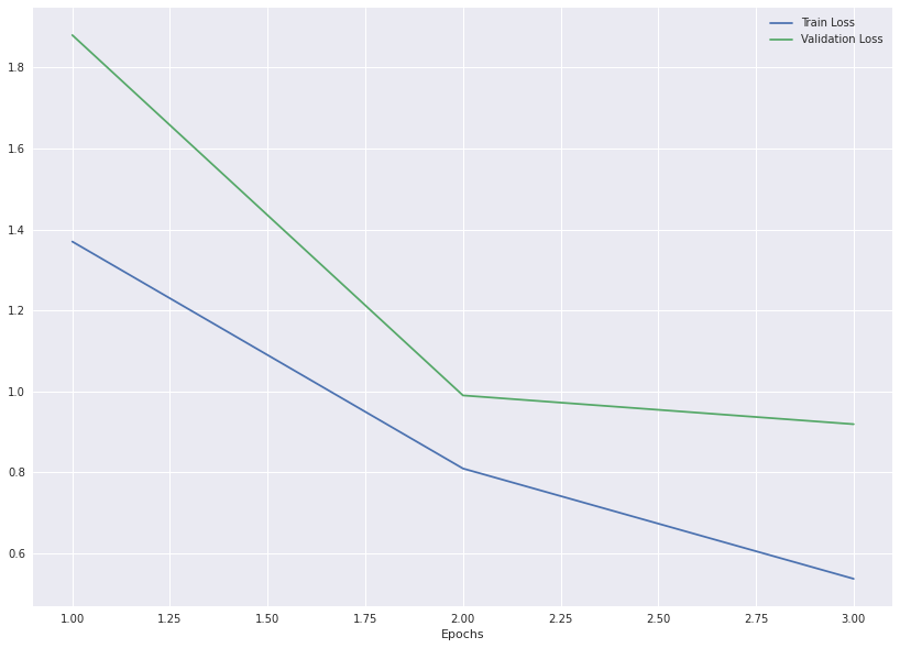
Both the training and the test losses seems to converge indicating the the fine-tuning was a success.
train_losses = [1.37, 0.8095, 0.5371]
val_losses = [1.88, 0.99, 0.919]

def plot_losses(train_losses, val_losses, epochs=3):
    df = pd.DataFrame(train_losses, columns =['Train Loss'])
    df['Validation Loss'] = val_losses
    df['Epochs'] = list(range(1,epochs+1))

    with plt.style.context('seaborn'):

        df.plot(x='Epochs',y=['Train Loss', 'Validation Loss'], figsize=(14,10))


plot_losses(train_losses, val_losses, epochs=3)
2.4 Evaluation
Load the fine tuned model
import torch
from transformers import AutoTokenizer,BertTokenizerFast

tokenizer = AutoTokenizer.from_pretrained('bert-base-uncased')

model = torch.load("../SQuAD_fine-tuned-BERT1",map_location=torch.device('cpu'))
model.eval()
print("Fine-tuned Model loaded!")
Fine-tuned Model loaded!
2.4.1 Predictions
Class Predict -Generates the answer for the query and context. Akso, computes F1 score which tells the average word overlap between predicted and ground-truth answers, which can ensure both of precision and recall rate are optimized at the same time.
def normalize_text(text):
    """Removing articles and punctuation, and standardizing whitespace are all typical text processing steps."""

    text = text.lower()

    exclude = set(string.punctuation)
    text = "".join(ch for ch in text if ch not in exclude)

    regex = re.compile(r"\b(a|an|the)\b", re.UNICODE)
    text = re.sub(regex, " ", text)

    text = " ".join(text.split())

    return text

class Predict:
    def get_answer(self, context, query):

        inputs = tokenizer.encode_plus(query, context, return_tensors='pt')

        outputs = model(**inputs)
        answer_start = torch.argmax(outputs[0])  # get the most likely beginning of answer with the argmax of the score
        answer_end = torch.argmax(outputs[1]) + 1

        answer = tokenizer.convert_tokens_to_string(tokenizer.convert_ids_to_tokens(inputs['input_ids'][0][answer_start:answer_end]))

        return answer

    def compute_f1(self, prediction, truth):
        pred_tokens = normalize_text(prediction).split()
        truth_tokens = normalize_text(truth).split()

        if len(pred_tokens) == 0 or len(truth_tokens) == 0:
            return int(pred_tokens == truth_tokens)

        common_tokens = set(pred_tokens) & set(truth_tokens)

        if len(common_tokens) == 0:
            return 0

        prec = len(common_tokens) / len(pred_tokens)
        rec = len(common_tokens) / len(truth_tokens)

        return 2 * (prec * rec) / (prec + rec)
def give_an_answer(context,query,answer, skip_score=False):
    infer = Predict()
    prediction = infer.get_answer(context,query)
    f1_score = infer.compute_f1(prediction, answer)

    print(f"Question: {query}")
    print(f"Prediction: {(prediction)}")
    print(f"True Answer: {(answer)}")
    if not skip_score:
        print(f"F1: {f1_score}")
    print("\n")
Here I give some examples to my model to see how well I trained it. I started with more easier examples and then I gave it more complex ones.
As you can see the model predicted all the answers correct in a very small an easy example.
context = "Hi! My name is Nidhin and I am 23 years old. I used to live in North of India, but now I moved on to Boulder in United States."

queries = ["How old is Nidhin?",
           "Where Nidhin used to live?",
           "Where does Nidhin live now?"
          ]
answers = ["23",
           "North of India",
           "Boulder in United States"
          ]

for q,a in zip(queries,answers):
    give_an_answer(context,q,a)
Question: How old is Nidhin?
Prediction: 23 years old.
True Answer: 23
F1: 0.5


Question: Where Nidhin used to live?
Prediction: north of india,
True Answer: North of India
F1: 1.0


Question: Where does Nidhin live now?
Prediction: boulder in united states.
True Answer: Boulder in United States
F1: 1.0
Here I took some text from Wikipedia to test my model. I observed that for questions that requires an answer with more than one entities, that in the context are seperated by comma, the model return only the first one.
context = """ Queen are a British rock band formed in London in 1970. Their classic line-up was Freddie Mercury (lead vocals, piano),
            Brian May (guitar, vocals), Roger Taylor (drums, vocals) and John Deacon (bass). Their earliest works were influenced
            by progressive rock, hard rock and heavy metal, but the band gradually ventured into more conventional and radio-friendly
            works by incorporating further styles, such as arena rock and pop rock. """

queries = ["When did Queen found?",
           "Who were the members of Queen band?",
           "What kind of band they are?"
          ]
answers = ["1970",
           "Freddie Mercury, Brian May, Roger Taylor and John Deacon",
           "arena rock and pop rock"
          ]

for q,a in zip(queries,answers):
    give_an_answer(context,q,a)
Question: When did Queen found?
Prediction: 1970.
True Answer: 1970
F1: 1.0


Question: Who were the members of Queen band?
Prediction: freddie mercury
True Answer: Freddie Mercury, Brian May, Roger Taylor and John Deacon
F1: 0.3636363636363636


Question: What kind of band they are?
Prediction: conventional and radio - friendly
True Answer: arena rock and pop rock
F1: 0.22222222222222224
On closer inspection I observed that this was due to the brackets that exists in the contxt. I figured model was thinking that the answer is complete as soon as it observed a bracket with multiple entities. So i remove them and test again.. and it works.
context = """ Queen are a British rock band formed in London in 1970. Their classic line-up was Freddie Mercury,
            Brian May, Roger Taylor and John Deacon (bass). Their earliest works were influenced
            by progressive rock, hard rock and heavy metal, but the band gradually ventured into more conventional and radio-friendly
            works by incorporating further styles, such as arena rock and pop rock. """

queries = [
           "Who were the members of Queen band?",
           ]
answers = [
           "Freddie Mercury, Brian May, Roger Taylor and John Deacon",
          ]

for q,a in zip(queries,answers):
    give_an_answer(context,q,a)
Question: Who were the members of Queen band?
Prediction: freddie mercury, brian may, roger taylor and john deacon
True Answer: Freddie Mercury, Brian May, Roger Taylor and John Deacon
F1: 1.0
Even for arithmetic answers and with questions that have the same words as the context, model performed quite well.
context = """  Mount Everest is Earth's highest mountain above sea level, located in the Mahalangur Himalayan
               sub-range of the Himalayas. The China–Nepal border runs across its summit point. Its
               elevation (snow height) of 8,848.86 m (29,031.7 ft) was most recently established in 2020
               by the Chinese and Nepali authorities. The first recorded efforts to reach Everest's summit
               were made by British mountaineers. As Nepal did not allow foreigners to enter the country at
               the time, the British made several attempts on the north ridge route from the Tibetan side. """

queries = [
           "How high is Everest?",
           "Where is Everest located?",
           "When was its elevation recently established?"
          ]

answers = [
           "8,848.86 m (29,031.7 ft)",
           "mahalangur himalayan sub-range",
           "2020"
          ]

for q,a in zip(queries,answers):
    give_an_answer(context,q,a)
Question: How high is Everest?
Prediction: 8, 848. 86 m ( 29, 031. 7 ft )
True Answer: 8,848.86 m (29,031.7 ft)
F1: 0.3333333333333333


Question: Where is Everest located?
Prediction: mahalangur himalayan sub - range of the himalayas.
True Answer: mahalangur himalayan sub-range
F1: 0.4444444444444444


Question: When was its elevation recently established?
Prediction: 2020
True Answer: 2020
F1: 1.0
I decided to test some arithmetic answers with confusing questions. These questions didn;t have the exact same words as the context, still model performed quite well except for one case. It couldn’t give the height in terms of metres. I think the model might not have the repersentation of m being metres here.
queries = [
           "How tall is Everest?",
           "How many metres is Everest?",
           "How many ft is Everest?",
           "How much high is Everest?",
           "How big is Everest?"
          ]

answers = [
           "8,848.86 m (29,031.7 ft)",
           "8,848.86 m",
           "29,031.7 ft",
           "8,848.86 m (29,031.7 ft)",
           "8,848.86 m (29,031.7 ft)"
          ]

for q,a in zip(queries,answers):
    give_an_answer(context,q,a,skip_score=True)
Question: How tall is Everest?
Prediction: 8, 848. 86 m ( 29, 031. 7 ft )
True Answer: 8,848.86 m (29,031.7 ft)


Question: How many metres is Everest?
Prediction: 29, 031. 7 ft )
True Answer: 8,848.86 m


Question: How many ft is Everest?
Prediction: 29, 031. 7 ft )
True Answer: 29,031.7 ft


Question: How much high is Everest?
Prediction: 8, 848. 86 m ( 29, 031. 7 ft )
True Answer: 8,848.86 m (29,031.7 ft)


Question: How big is Everest?
Prediction: 8, 848. 86 m ( 29, 031. 7 ft )
True Answer: 8,848.86 m (29,031.7 ft)
Finally, I decided to put a lot of arithmetic answers in the context to make it harder for the model. Still, the model performed very well.
context = """  Mount Everest is Earth's highest mountain above sea level, located in the Mahalangur Himalayan
               sub-range of the Himalayas. The China–Nepal border runs across its summit point. Its
               elevation (snow height) of 8,848.86 m (29,031.7 ft) was most recently established in 2020
               by the Chinese and Nepali authorities. After the first reconnaissance expedition by the British
               in 1921 reached 7,000 m (22,970 ft) on the North Col, the 1922 expedition pushed the north ridge
               route up to 8,320 m (27,300 ft), marking the first time a human had climbed above 8,000 m (26,247 ft). """

queries = [
           "How many metres is Everest?",
           "How far did British reach in 1921?",
           "How much did the first human go?"
          ]

answers = [
           "8,848.86 m (29,031.7 ft)",
           "7,000 m (22,970 ft)",
           "8,000 m (26,247 ft)"
          ]

for q,a in zip(queries,answers):
    give_an_answer(context,q,a,skip_score=True)
Question: How many metres is Everest?
Prediction: 8, 848. 86 m ( 29, 031. 7 ft )
True Answer: 8,848.86 m (29,031.7 ft)


Question: How far did British reach in 1921?
Prediction: 7, 000 m ( 22, 970 ft )
True Answer: 7,000 m (22,970 ft)


Question: How much did the first human go?
Prediction: 8, 000 m
True Answer: 8,000 m (26,247 ft)
Visualizing
One of the best ways to interpret and validate the results here would be to unravel the attention head themselves. Here I try to visualize what portion of context the model focuses on when asked a query.I use bertviz to interpret and visualize the attention heads.
Note: Due to having render issues of the output of bertviz when uploaded to github, I am attaching the images of the output below.
# !pip install bertviz
from bertviz import head_view, model_view
from transformers import BertTokenizer, BertModel, BertForQuestionAnswering
from bertviz.neuron_view import show

model_version = 'bert-base-uncased'
model = BertForQuestionAnswering.from_pretrained('../BERT-zip/', output_attentions=True)
context = "Hi! My name is nidhin and I am 23 years old. I used to live in North of India, but now I moved on to Boulder in United States."

queries = ["How old is nidhin ?",
           "Where nidhin used to live?",
           "Where does nidhin live now?"
          ]
answers = ["23",
           "North of India",
           "Boulder in United States"
          ]


def show_attention(query, context, show_attention=True, show_model=False):
    inputs = tokenizer.encode_plus(query, context, return_tensors='pt')
    input_ids = inputs['input_ids']
    token_type_ids = inputs['token_type_ids']

    attention = model(input_ids, token_type_ids=token_type_ids)[-1]

    sentence_b_start = token_type_ids[0].tolist().index(1)
    input_id_list = input_ids[0].tolist() # Batch index 0
    tokens = tokenizer.convert_ids_to_tokens(input_id_list)
    if show_model:
        model_view(attention, tokens, sentence_b_start)
        return None

    if show_attention:
        head_view(attention, tokens, sentence_b_start)
        return None
show_attention(queries[0], context, show_attention=True)
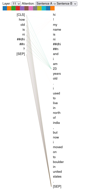
I also try visualizing whats going inside of each of the attention heads. Ignore the attention of
show_attention(queries[0], context, show_model=True)
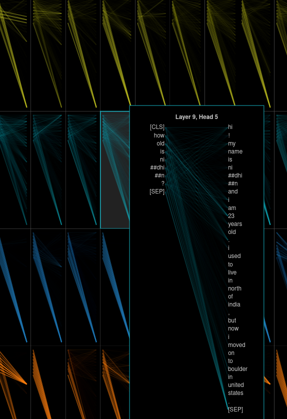
Saving Predictions for comparison study
Just saving the predictions on the dev set for comparison study in SQuAD-EDA.ipynb
tokenizer = AutoTokenizer.from_pretrained('bert-base-uncased')

model = torch.load("../SQuAD_fine-tuned-BERT1",map_location=torch.device('cpu'))
model.eval()
print("Fine-tuned Model loaded!")

DEV_DIR = Path('squad/dev-v2.0.json')
Fine-tuned Model loaded!
def load_data(path, data_type=None):

    print(f"Processing {data_type}...")
    with open(path, 'rb') as f:
        squad_dict = json.load(f)

    texts, queries, lookup = [], [], [], []

    for group in squad_dict['data']:
        for passage in group['paragraphs']:
            context = passage['context']

            for qa in passage['qas']:
                question = qa['question']
                idx = qa["id"]
                lookup.append(idx)
                texts.append(context)
                queries.append(question)
    print("\t Completed!\n")
    return texts, queries, lookup

val_texts, val_queries, lookup = load_data(path=DEV_DIR, data_type="Test")
Processing Test...
	 Completed!
dev_pred = dict()
SAVE_NAME = "SQuADv2-dev-predictions.json"
def get_answer(context, query):

    inputs = tokenizer.encode_plus(query, context, return_tensors='pt')

    outputs = model(**inputs)
    answer_start = torch.argmax(outputs[0])
    answer_end = torch.argmax(outputs[1]) + 1

    answer = tokenizer.convert_tokens_to_string(tokenizer.convert_ids_to_tokens(inputs['input_ids'][0][answer_start:answer_end]))

    return answer

for i in range(len(val_texts)):
    if i%1000==0:
        print(i, end='\r')
    dev_pred[lookup[i]] = get_answer(val_texts[i], val_queries[i])

with open(SAVE_NAME, 'w') as fp:
    json.dump(data, fp)
1100

Predictions on dev saved.. SQuADv2-dev-predictions.json
Discussion
I started with the absolute fundamentals by implementing BERT completely from scratch. Even though my implementation of BERT wasn’t the most efficient, but still it converged nicely and we were able see semantic relationships in the map of word embeddings. Using a pre-trained version and fine-tuning took a lot of time for me. Since, the model had about 109M parameters, it comes amongst the big model and training it was not easy. It is however, fascinating to see how the fine-tuning just converged so rapidly and the pre-trained model was now able to do the task of question-answering which was completely different from that task it was trained on, in just 3 epochs.
Since one of the huge challenges faced in NLP is the lack of annotated data and on top of that, we require huge models to perform well on different tasks. Unsupervised pretraining methods like BERT which leaved a huge scope of improvement when it comes to transfer learning, bridges this gap. I do think that this is the way to go in NLP especially, inorder to generate general purpose language representations which could be used in fine-tuning for specific tasks.
There is still lots of scope in terms of fine-tuning these methods but at the end I believe that we need to go with research question of defining unsupervised approach based pre-text tasks like masking in BERT, for learning improved, meaningful and generalizable language representations,
Refernces
[1] Devlin, Jacob, et al. "Bert: Pre-training of deep bidirectional transformers for language understanding." arXiv preprint arXiv:1810.04805 (2018).

[2] Wolf, Thomas, et al. "Huggingface's transformers: State-of-the-art natural language processing." arXiv preprint arXiv:1910.03771 (2019).

[3] Rajpurkar, Pranav, et al. "Squad: 100,000+ questions for machine comprehension of text." arXiv preprint arXiv:1606.05250 (2016).

[4] Hyugen AI - Transformers in Pytorch Tutorial

[5] BERT Explained: A Complete Guide with Theory and Tutorial, TowardsML

[6] Alexaapo - BERT based pretrained model using SQuAD 2.0 Dataset