In this notebook, I’ll be implementing some of architectures that we studied in the last few lectures for cifar-10 classification. Specifically, I’ll be comparing 3 methods:

[1] GoogLeNet: Szegedy, Christian, et al. “Going deeper with convolutions.” Proceedings of the IEEE conference on computer vision and pattern recognition. 2015.

[2] ResNet: He, Kaiming, et al. “Deep residual learning for image recognition.” Proceedings of the IEEE conference on computer vision and pattern recognition. 2016.

[3] Preact-ResNet (improved resnet): He, Kaiming, et al. “Identity mappings in deep residual networks.” European conference on computer vision. Springer, Cham, 2016.

import os
import argparse
import pickle

import matplotlib.pyplot as plt

from sklearn import decomposition
from sklearn import manifold
from sklearn.metrics import confusion_matrix
from sklearn.metrics import ConfusionMatrixDisplay

import torch
import torch.nn as nn
import torch.optim as optim
import torch.nn.functional as F
import torch.backends.cudnn as cudnn

from torchsummary import summary
import torchvision
import torchvision.transforms as transforms

1. CIFAR-10 Dataset

While the actual implementation of above mentioned models were mostly trained on Imagenet dataset (~1.2 million images). Due to computational time constraints, I plan on using a lighter dataset like the CIFAR-10 dataset, which is a classical computer-vision dataset for object recognition case study.

Below function will download CIFAR10 dataset from the official PyTorch datasets

When downloaded, CIFAR-10 data will consist of thousands of RGB images. The preprocessing of CIFAR-10 will need the following steps:

Obtaining the mean and standard deviation of the data so it can be normalized. Each image in the dataset is made up of three channels RGB (red, green and blue). Therefore, means and standard deviations for each of the color channels needs to calculated independently. The mean and standard deviation values that is used to normalize are standard and publicly available. I just straightaway define them.

I apply the following set of specific augmentations to our CIFAR-10 dataset:

RandomHorizontalFlip - This, with a probability of 0.5 as specified, flips the image horizontally.
RandomCrop - takes a random 32x32 square crop of the image.
ToTensor - converts image from a PIL image into a PyTorch tensor.
Normalize - this subtracts the image pixels channel-wise with its mean and divides by the given standard deviation.

device = 'cuda' if torch.cuda.is_available() else 'cpu'
print('==> Preparing data..')

# Data Augmentations ---------------------------------------------------------
transform_train = transforms.Compose([
    transforms.RandomCrop(32, padding=4),
    transforms.RandomHorizontalFlip(),
    transforms.ToTensor(),
    transforms.Normalize((0.4914, 0.4822, 0.4465), (0.2023, 0.1994, 0.2010)),
])

transform_test = transforms.Compose([
    transforms.ToTensor(),
    transforms.Normalize((0.4914, 0.4822, 0.4465), (0.2023, 0.1994, 0.2010)),
])
# ------------------------------------------------------------------------------


# Downloading train-set of CIFAR-10 (with a batch-size of 128)
trainset = torchvision.datasets.CIFAR10(
    root='./data', train=True, download=True, transform=transform_train)
trainloader = torch.utils.data.DataLoader(
    trainset, batch_size=128, shuffle=True, num_workers=2)


# Downloading test-set CIFAR-10 (with a batch-size of 128)
testset = torchvision.datasets.CIFAR10(
    root='./data', train=False, download=True, transform=transform_test)
testloader = torch.utils.data.DataLoader(
    testset, batch_size=100, shuffle=False, num_workers=2)

classes = ('plane', 'car', 'bird', 'cat', 'deer',
           'dog', 'frog', 'horse', 'ship', 'truck')

==> Preparing data..
Files already downloaded and verified
Files already downloaded and verified

print(f'Number of training examples: {len(trainset)}')
print(f'Number of testing examples: {len(testset)}')

Number of training examples: 50000
Number of testing examples: 10000

1.1 Data analysis (Abridged)

I have already covered exploratoary data analysis in my previous notebook, so I won’t be going all over it again. Instead, here’s some of the key data-related statistics and its visualization.

print("\nNumber of classes:", len(trainset.classes))
print("Classes:", trainset.classes)

Number of classes: 10
Classes: ['airplane', 'automobile', 'bird', 'cat', 'deer', 'dog', 'frog', 'horse', 'ship', 'truck']

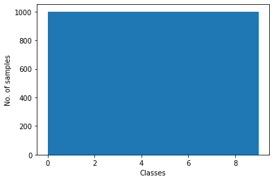
print("Distribution of classes (Test)")
plt.hist(testset.targets)
plt.xlabel("Classes")
plt.ylabel("No. of samples")
plt.show()

Distribution of classes (Test)

png

print("Distribution of classes (Train)")
plt.hist(trainset.targets)
plt.xlabel("Classes")
plt.ylabel("No. of samples")
plt.show()

Distribution of classes (Train)

png

CIFAR10 is a highly balanced dataset with equal distribution in each class as can be seen from above histograms.

1.2 Visualization

Here, I create a function to plot some images in our dataset to see what they actually look like. Note that by default PyTorch handles images that are arranged [channel, height, width], but matplotlib expects images to be [height, width, channel], hence we need to permute our images before plotting them.

from torchvision.utils import make_grid
import ipyplot

def show(imgs):
    plt.rcParams["figure.figsize"] = (10,20)
    plt.imshow(imgs.permute(1, 2, 0))
    plt.axis('off')
    plt.show()

labels_set = trainset.targets[:30]
textual_labels = [trainset.classes[labels_set[i]] for i in range(30)]
ipyplot.plot_class_representations(trainset.data[:30],textual_labels)

airplane

automobile

bird

cat

deer

dog

frog

horse

ship

truck

airplane

automobile

bird

cat

deer

dog

frog

horse

ship

truck

2. Image Recognition Architectures

2.1 GoogLeNet

The LeNet-5 convolutional neural network (introduced in 1998 by Yann LeCun et al. in the paper “Gradient-Based Learning Applied To Document Recognition”) was the first paper which showed utilisation of convolutional neural networks for the computer vision task of image classification. Following that in 2012 - AlexNet came (I covered in my previous report), a convolutional neural network architecture introduced the composition of consecutively stacked convolutional layers. The creators of AlexNet trained the network using graphical processing units (GPUs).

Following these 2 papers, efficient computing resources and intuitive CNN architectures led to the rapid development of competetive solutions to lot of computer vision tasks. Although, researchers discovered that an increase of layers and units within a network led to a significant performance gain. But they also foudn out that - increasing the layers to create more extensive networks came at a cost. Large networks are prone to overfitting and suffer from either exploding or vanishing gradient problem.

The GoogLeNet architecture (introduced in 2015 - “Going Deeper with Convolutions”) solved most of the problems that large networks faced, mainly through the Inception module’s utilisation.

Figure. Inception module

At the time researchers were a bit confused on exactly what kernel sizes to use for their convolutional networks. The Inception module is a neural network architecture that leverages feature detection at different scales through convolutions with different kernel sizes and reduced the computational cost of training an extensive network through dimensional reduction.

Below I implement the inception module with a slight modiifcation of adding batch-normalization to stabilize the training (the original implementation doesn’t contain batch-normalization):

class Inception(nn.Module):
    def __init__(self, in_planes, n1x1, n3x3red, n3x3, n5x5red, n5x5, pool_planes):
        super(Inception, self).__init__()
        # 1x1 conv branch
        self.b1 = nn.Sequential(
            nn.Conv2d(in_planes, n1x1, kernel_size=1),
            nn.BatchNorm2d(n1x1),
            nn.ReLU(True),
        )

        # 1x1 conv -> 3x3 conv branch
        self.b2 = nn.Sequential(
            nn.Conv2d(in_planes, n3x3red, kernel_size=1),
            nn.BatchNorm2d(n3x3red),
            nn.ReLU(True),
            nn.Conv2d(n3x3red, n3x3, kernel_size=3, padding=1),
            nn.BatchNorm2d(n3x3),
            nn.ReLU(True),
        )

        # 1x1 conv -> 5x5 conv branch
        self.b3 = nn.Sequential(
            nn.Conv2d(in_planes, n5x5red, kernel_size=1),
            nn.BatchNorm2d(n5x5red),
            nn.ReLU(True),
            nn.Conv2d(n5x5red, n5x5, kernel_size=3, padding=1),
            nn.BatchNorm2d(n5x5),
            nn.ReLU(True),
            nn.Conv2d(n5x5, n5x5, kernel_size=3, padding=1),
            nn.BatchNorm2d(n5x5),
            nn.ReLU(True),
        )

        # 3x3 pool -> 1x1 conv branch
        self.b4 = nn.Sequential(
            nn.MaxPool2d(3, stride=1, padding=1),
            nn.Conv2d(in_planes, pool_planes, kernel_size=1),
            nn.BatchNorm2d(pool_planes),
            nn.ReLU(True),
        )

    def forward(self, x):
        y1 = self.b1(x)
        y2 = self.b2(x)
        y3 = self.b3(x)
        y4 = self.b4(x)
        return torch.cat([y1,y2,y3,y4], 1)

Figure. GoogLeNet architecture

The GoogLeNet architecture consists of 22 layers (27 layers including pooling layers), and part of these layers are a total of 9 inception modules. Following is the implementation of whole GoogLeNet architecture:

class GoogLeNet(nn.Module):
    def __init__(self):
        super(GoogLeNet, self).__init__()
        self.pre_layers = nn.Sequential(
            nn.Conv2d(3, 192, kernel_size=3, padding=1),
            nn.BatchNorm2d(192),
            nn.ReLU(True),
        )

        self.a3 = Inception(192,  64,  96, 128, 16, 32, 32)
        self.b3 = Inception(256, 128, 128, 192, 32, 96, 64)

        self.maxpool = nn.MaxPool2d(3, stride=2, padding=1)

        self.a4 = Inception(480, 192,  96, 208, 16,  48,  64)
        self.b4 = Inception(512, 160, 112, 224, 24,  64,  64)
        self.c4 = Inception(512, 128, 128, 256, 24,  64,  64)
        self.d4 = Inception(512, 112, 144, 288, 32,  64,  64)
        self.e4 = Inception(528, 256, 160, 320, 32, 128, 128)

        self.a5 = Inception(832, 256, 160, 320, 32, 128, 128)
        self.b5 = Inception(832, 384, 192, 384, 48, 128, 128)

        self.avgpool = nn.AvgPool2d(8, stride=1)
        self.linear = nn.Linear(1024, 10)

    def forward(self, x):
        out = self.pre_layers(x)
        out = self.a3(out)
        out = self.b3(out)
        out = self.maxpool(out)
        out = self.a4(out)
        out = self.b4(out)
        out = self.c4(out)
        out = self.d4(out)
        out = self.e4(out)
        out = self.maxpool(out)
        out = self.a5(out)
        out = self.b5(out)
        out = self.avgpool(out)
        out = out.view(out.size(0), -1)
        out = self.linear(out)
        return out
    
g_net = GoogLeNet()
g_net = g_net.to(device)

Hyper-parameters:

I set the optimization criterion to Cross Entropy - a standard classification loss.
I initialize stochastic gradient descent (SGD) optimizer with a learning rate of 1e-1.
Additionally, I apply a learning rate scheduler which reduces the learning rate using cosine annealing if the performance stagnates.

if device == 'cuda':
    net = torch.nn.DataParallel(g_net)
    cudnn.benchmark = True

criterion = nn.CrossEntropyLoss()
optimizer = optim.SGD(g_net.parameters(), lr=0.1, momentum=0.9, weight_decay=5e-4)
scheduler = torch.optim.lr_scheduler.CosineAnnealingLR(optimizer, T_max=200)

best_acc = 0  # best test accuracy
start_epoch = 0  # start from epoch 0 or last checkpoint epoch

Testing

In the following function, I’ll be switching off the gradient computation using torch.no_grad and doing the evaluation on test set. I do the following:

Compute the loss and accuracy over the test set.
Print the logs of evaluation if promted (controlled with log_epochs).
Save the best performing model checkpoint

def test(net, epoch, total_epochs, log_epochs=None, save_ckpt=None):
    global best_acc
    net.eval()
    test_loss = 0
    correct = 0
    total = 0
    with torch.no_grad():
        for batch_idx, (inputs, targets) in enumerate(testloader):
            inputs, targets = inputs.to(device), targets.to(device)
            outputs = net(inputs)
            loss = criterion(outputs, targets)  # test loss
            test_loss += loss.item()
            _, predicted = outputs.max(1)
            total += targets.size(0)   # total predictions
            correct += predicted.eq(targets).sum().item()  # correct predictions
        
        # Test-set evaluation logs     
        if epoch%log_epochs==0:
            print('\t     Test Loss: %.3f | Test Acc: %.3f%% (%d/%d)'
                  % (test_loss/(batch_idx+1), 100.*correct/total, correct, total))

    # Save checkpoint.
    acc = 100.*correct/total
    if acc > best_acc:
        state = {
            'net': net.state_dict(),
            'acc': acc,
            'epoch': epoch,
        }
        if not os.path.isdir('checkpoint'):
            os.mkdir('checkpoint')
        torch.save(state, './checkpoint/save_ckpt.pth')
        best_acc = acc
    
    return test_loss, (100.*correct/total)

Training

The below function is used to train the GoogLeNet. After each forward-backward propagation, it accumulates the per-batch losses and accuracies and prints the logs if prompted (controlled with log_epochs).

def train(net, epoch, total_epochs, log_epochs=None):
    
    net.train()
    train_loss = 0
    correct = 0
    total = 0
    for batch_idx, (inputs, targets) in enumerate(trainloader):
        inputs, targets = inputs.to(device), targets.to(device)
        optimizer.zero_grad()
        outputs = net(inputs)
        loss = criterion(outputs, targets)
        loss.backward()
        optimizer.step()

        train_loss += loss.item()
        _, predicted = outputs.max(1)
        total += targets.size(0)
        correct += predicted.eq(targets).sum().item()
    train_loss/=(batch_idx+1)
    if epoch%log_epochs==0:
            print(f'Epoch: {epoch} -> Train Loss: {train_loss:.3f} | Train Acc: {100.*correct/total} ({correct}/{total})')

    return train_loss, (100.*correct/total)

Now that we have all the components for training our implementation of GoogLeNet ready, we can start the training procedure. For each iteration, I’m training GoogLeNet on the training samples and computing the loss and accuracy values. It is followed by evaluation on the test-set. All the loss and accuracy values are stored and dumped for later use.

%%capture gnet_stdout 

gnet_logs = {'tl':[], 'ta':[], 'vl':[], 'va':[]}
total_epochs = 200

for epoch in range(start_epoch, start_epoch+total_epochs):
    
    train_loss, train_acc = train(g_net, epoch, total_epochs, log_epochs=10)
    test_loss, test_acc = test(g_net, epoch, total_epochs, log_epochs=10)
    
    train_loss/=len(trainloader)
    test_loss/=len(testloader)
    gnet_logs['tl'].append(train_loss)
    gnet_logs['ta'].append(train_acc)
    gnet_logs['vl'].append(test_loss)
    gnet_logs['va'].append(test_acc)
    scheduler.step()

# save logs to file
with open('Gnet_logs.pkl', 'wb') as f:
    pickle.dump(gnet_logs, f)
        

gnet_stdout()

Epoch: 0 -> Train Loss: 1.580 | Train Acc: 41.714 (20857/50000)
	     Test Loss: 1.282 | Test Acc: 54.470% (5447/10000)
Epoch: 10 -> Train Loss: 0.420 | Train Acc: 85.678 (42839/50000)
	     Test Loss: 0.621 | Test Acc: 79.500% (7950/10000)
Epoch: 20 -> Train Loss: 0.341 | Train Acc: 88.306 (44153/50000)
	     Test Loss: 0.554 | Test Acc: 81.830% (8183/10000)
Epoch: 30 -> Train Loss: 0.305 | Train Acc: 89.578 (44789/50000)
	     Test Loss: 0.650 | Test Acc: 79.600% (7960/10000)
Epoch: 40 -> Train Loss: 0.292 | Train Acc: 89.894 (44947/50000)
	     Test Loss: 0.488 | Test Acc: 84.040% (8404/10000)
Epoch: 50 -> Train Loss: 0.264 | Train Acc: 90.854 (45427/50000)
	     Test Loss: 0.763 | Test Acc: 77.520% (7752/10000)
Epoch: 60 -> Train Loss: 0.243 | Train Acc: 91.684 (45842/50000)
	     Test Loss: 0.595 | Test Acc: 81.030% (8103/10000)
Epoch: 70 -> Train Loss: 0.230 | Train Acc: 92.022 (46011/50000)
	     Test Loss: 0.697 | Test Acc: 79.470% (7947/10000)
Epoch: 80 -> Train Loss: 0.205 | Train Acc: 92.918 (46459/50000)
	     Test Loss: 0.639 | Test Acc: 81.260% (8126/10000)
Epoch: 90 -> Train Loss: 0.182 | Train Acc: 93.718 (46859/50000)
	     Test Loss: 0.673 | Test Acc: 80.030% (8003/10000)
Epoch: 100 -> Train Loss: 0.154 | Train Acc: 94.742 (47371/50000)
	     Test Loss: 0.476 | Test Acc: 85.760% (8576/10000)
Epoch: 110 -> Train Loss: 0.124 | Train Acc: 95.772 (47886/50000)
	     Test Loss: 0.420 | Test Acc: 87.380% (8738/10000)
Epoch: 120 -> Train Loss: 0.102 | Train Acc: 96.636 (48318/50000)
	     Test Loss: 0.356 | Test Acc: 89.270% (8927/10000)
Epoch: 130 -> Train Loss: 0.071 | Train Acc: 97.654 (48827/50000)
	     Test Loss: 0.652 | Test Acc: 82.360% (8236/10000)
Epoch: 140 -> Train Loss: 0.052 | Train Acc: 98.326 (49163/50000)
	     Test Loss: 0.295 | Test Acc: 91.370% (9137/10000)
Epoch: 150 -> Train Loss: 0.021 | Train Acc: 99.444 (49722/50000)
	     Test Loss: 0.249 | Test Acc: 93.090% (9309/10000)
Epoch: 160 -> Train Loss: 0.003 | Train Acc: 99.994 (49997/50000)
	     Test Loss: 0.159 | Test Acc: 95.180% (9518/10000)
Epoch: 170 -> Train Loss: 0.003 | Train Acc: 100.0 (50000/50000)
	     Test Loss: 0.152 | Test Acc: 95.150% (9515/10000)
Epoch: 180 -> Train Loss: 0.003 | Train Acc: 99.998 (49999/50000)
	     Test Loss: 0.153 | Test Acc: 95.120% (9512/10000)
Epoch: 190 -> Train Loss: 0.002 | Train Acc: 100.0 (50000/50000)
	     Test Loss: 0.149 | Test Acc: 95.340% (9534/10000)

2.2 ResNet-18

Following GoogLeNet, lot of researchers starting working with deeper and more complex models. One of the complication they faced with going deep with convlutional nets was that - with the network depth increasing, accuracy gets saturated and then degrades rapidly.

In an attempt to solve this, a set of researchers came up with the following idea: Instead of learning a direct mapping of \(x\rightarrow y\) with a function \(H(x)\) (A few stacked non-linear layers). Let us define the residual function using \(F(x) = H(x) — x\), which can be reframed into \(H(x) = F(x)+x\), where \(F(x)\) and \(x\) represents the stacked non-linear layers and the identity function(input=output) respectively.

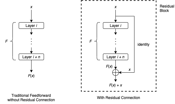
The ResNet-18 architecture uses such residual connections such that the input passed via the shortcut matches is resized to dimensions of the main path’s output. Following shows the overall structure of ResNet-18 architecture:

Here I implement the ResNet-18 architecture. The Basicblock defines the block before and after which there’ll be residual connections (shortcut). The ResNet classs compiles several such Basicblock(s) and adds residuals to them (resizes the residual inputs if required).

# Basic block before and after which there are shortcut connections. 
# Batch-norm is a modification I added for stability.
class BasicBlock(nn.Module):
    expansion = 1
    def __init__(self, in_planes, planes, stride=1):
        super(BasicBlock, self).__init__()
        self.conv1 = nn.Conv2d(
            in_planes, planes, kernel_size=3, stride=stride, padding=1, bias=False)
        self.bn1 = nn.BatchNorm2d(planes)
        self.conv2 = nn.Conv2d(planes, planes, kernel_size=3,
                               stride=1, padding=1, bias=False)
        self.bn2 = nn.BatchNorm2d(planes)

        self.shortcut = nn.Sequential()
        if stride != 1 or in_planes != self.expansion*planes:
            self.shortcut = nn.Sequential(
                nn.Conv2d(in_planes, self.expansion*planes,
                          kernel_size=1, stride=stride, bias=False),
                nn.BatchNorm2d(self.expansion*planes)
            )

    def forward(self, x):
        out = F.relu(self.bn1(self.conv1(x)))
        out = self.bn2(self.conv2(out))
        out += self.shortcut(x)
        out = F.relu(out)
        return out

# Resnet class
class ResNet(nn.Module):
    def __init__(self, block, num_blocks, num_classes=10):
        super(ResNet, self).__init__()
        self.in_planes = 64

        self.conv1 = nn.Conv2d(3, 64, kernel_size=3,
                               stride=1, padding=1, bias=False)
        self.bn1 = nn.BatchNorm2d(64)
        self.layer1 = self._make_layer(block, 64, num_blocks[0], stride=1)
        self.layer2 = self._make_layer(block, 128, num_blocks[1], stride=2)
        self.layer3 = self._make_layer(block, 256, num_blocks[2], stride=2)
        self.layer4 = self._make_layer(block, 512, num_blocks[3], stride=2)
        self.linear = nn.Linear(512*block.expansion, num_classes)
    
    # resizing the shortcuts with strides whenever required before adding them
    # to the main path 
    def _make_layer(self, block, planes, num_blocks, stride):
        strides = [stride] + [1]*(num_blocks-1)
        layers = []
        for stride in strides:
            layers.append(block(self.in_planes, planes, stride))
            self.in_planes = planes * block.expansion
        return nn.Sequential(*layers)

    def forward(self, x):
        out = F.relu(self.bn1(self.conv1(x)))
        out = self.layer1(out)
        out = self.layer2(out)
        out = self.layer3(out)
        out = self.layer4(out)
        out = F.avg_pool2d(out, 4)
        out = out.view(out.size(0), -1)
        out = self.linear(out)
        return out

# Initiating the resnet class with blocks as defined in the original paper.
def ResNet18():
    return ResNet(BasicBlock, [2, 2, 2, 2])

res_net = ResNet18()
res_net = res_net.to(device)

Hyperparameters

Same set of Hyperparameters are used as for fair-comparison

if device == 'cuda':
    net = torch.nn.DataParallel(res_net)
    cudnn.benchmark = True

criterion = nn.CrossEntropyLoss()
optimizer = optim.SGD(res_net.parameters(), lr=0.1, momentum=0.9, weight_decay=5e-4)
scheduler = torch.optim.lr_scheduler.CosineAnnealingLR(optimizer, T_max=200)

%%capture resnet_stdout

best_acc = 0  # best test accuracy
start_epoch = 0  # start from epoch 0 or last checkpoint epoch
total_epochs = 101

resnet_logs = {'tl':[], 'ta':[], 'vl':[], 'va':[]}

for epoch in range(start_epoch, start_epoch+total_epochs):
    
    train_loss, train_acc = train(res_net, epoch, total_epochs, log_epochs=10)
    test_loss, test_acc = test(res_net, epoch, total_epochs, log_epochs=10, save_ckpt="resnet")
    
    train_loss/=len(trainloader)
    test_loss/=len(testloader)
    resnet_logs['tl'].append(train_loss)
    resnet_logs['ta'].append(train_acc)
    resnet_logs['vl'].append(test_loss)
    resnet_logs['va'].append(test_acc)
    scheduler.step()

with open('resnet_logs.pkl', 'wb') as f:
    pickle.dump(resnet_logs, f)
    

resnet_stdout()

Epoch: 0 -> Train Loss: 2.043 | Train Acc: 26.122 (13061/50000)
	     Test Loss: 1.612 | Test Acc: 39.590% (3959/10000)
Epoch: 10 -> Train Loss: 0.507 | Train Acc: 82.658 (41329/50000)
	     Test Loss: 0.711 | Test Acc: 76.380% (7638/10000)
Epoch: 20 -> Train Loss: 0.391 | Train Acc: 86.676 (43338/50000)
	     Test Loss: 0.558 | Test Acc: 81.650% (8165/10000)
Epoch: 30 -> Train Loss: 0.348 | Train Acc: 88.074 (44037/50000)
	     Test Loss: 0.510 | Test Acc: 82.830% (8283/10000)
Epoch: 40 -> Train Loss: 0.322 | Train Acc: 89.028 (44514/50000)
	     Test Loss: 0.447 | Test Acc: 85.120% (8512/10000)
Epoch: 50 -> Train Loss: 0.304 | Train Acc: 89.698 (44849/50000)
	     Test Loss: 0.552 | Test Acc: 82.260% (8226/10000)
Epoch: 60 -> Train Loss: 0.284 | Train Acc: 90.42 (45210/50000)
	     Test Loss: 0.514 | Test Acc: 82.970% (8297/10000)
Epoch: 70 -> Train Loss: 0.262 | Train Acc: 91.034 (45517/50000)
	     Test Loss: 0.432 | Test Acc: 85.380% (8538/10000)
Epoch: 80 -> Train Loss: 0.240 | Train Acc: 91.824 (45912/50000)
	     Test Loss: 0.391 | Test Acc: 87.020% (8702/10000)
Epoch: 90 -> Train Loss: 0.216 | Train Acc: 92.568 (46284/50000)
	     Test Loss: 0.305 | Test Acc: 90.260% (9026/10000)
Epoch: 100 -> Train Loss: 0.185 | Train Acc: 93.634 (46817/50000)
	     Test Loss: 0.345 | Test Acc: 89.250% (8925/10000)

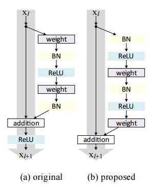
2.3 PreAct-R18 (Identity Mappings in Deep Residual Networks)

This is a follow-up work to the ResNet-18. As we discussed in the lecture, residual block can be represented with the equations \(y_l = h(x_l) + F(x_l, W_l)\); \(x_{l+1} = f(y_l)\), where \(x_l\) is the input to the \(l-th\) unit and \(x_{l+1}\) is the output of the \(l-th\) unit. In the original ResNet-18, \(h(x_l) = x_l\), \(f\) is ReLu, and \(F\) consists of 2-3 convolutional layers (basic-block based architecture) with BN and ReLU in between. In this, they propose a residual block with both \(h(x)\) and \(f(x)\) as identity mappings involving BN and ReLU before the actual convolutions for efficient training and better performance.

class PreActBlock(nn.Module):
    '''Pre-activation version of the BasicBlock. The modification is addition of BatchNorm and ReLU before convolutions'''
    expansion = 1

    def __init__(self, in_planes, planes, stride=1):
        super(PreActBlock, self).__init__()
        self.bn1 = nn.BatchNorm2d(in_planes)
        self.conv1 = nn.Conv2d(in_planes, planes, kernel_size=3, stride=stride, padding=1, bias=False)
        self.bn2 = nn.BatchNorm2d(planes)
        self.conv2 = nn.Conv2d(planes, planes, kernel_size=3, stride=1, padding=1, bias=False)

        if stride != 1 or in_planes != self.expansion*planes:
            self.shortcut = nn.Sequential(
                nn.Conv2d(in_planes, self.expansion*planes, kernel_size=1, stride=stride, bias=False)
            )

    def forward(self, x):
        out = F.relu(self.bn1(x))
        shortcut = self.shortcut(out) if hasattr(self, 'shortcut') else x
        out = self.conv1(out)
        out = self.conv2(F.relu(self.bn2(out)))
        out += shortcut
        return out

# Quite similar to the ResNet-18 class except it utilizes the modified PreActBlock
class PreActResNet(nn.Module):
    def __init__(self, block, num_blocks, num_classes=10):
        super(PreActResNet, self).__init__()
        self.in_planes = 64

        self.conv1 = nn.Conv2d(3, 64, kernel_size=3, stride=1, padding=1, bias=False)
        self.layer1 = self._make_layer(block, 64, num_blocks[0], stride=1)
        self.layer2 = self._make_layer(block, 128, num_blocks[1], stride=2)
        self.layer3 = self._make_layer(block, 256, num_blocks[2], stride=2)
        self.layer4 = self._make_layer(block, 512, num_blocks[3], stride=2)
        self.linear = nn.Linear(512*block.expansion, num_classes)

    def _make_layer(self, block, planes, num_blocks, stride):
        strides = [stride] + [1]*(num_blocks-1)
        layers = []
        for stride in strides:
            layers.append(block(self.in_planes, planes, stride))
            self.in_planes = planes * block.expansion
        return nn.Sequential(*layers)

    def forward(self, x):
        out = self.conv1(x)
        out = self.layer1(out)
        out = self.layer2(out)
        out = self.layer3(out)
        out = self.layer4(out)
        out = F.avg_pool2d(out, 4)
        out = out.view(out.size(0), -1)
        out = self.linear(out)
        return out

# Modified PreAct-ResNet-18
def PreActResNet18():
    return PreActResNet(PreActBlock, [2,2,2,2])


preres_net = PreActResNet18()
preres_net = preres_net.to(device)

Hyper-parameters

Same set of Hyperparameters are used as for fair-comparison

if device == 'cuda':
    net = torch.nn.DataParallel(preres_net)
    cudnn.benchmark = True

criterion = nn.CrossEntropyLoss()
optimizer = optim.SGD(preres_net.parameters(), lr=0.1, momentum=0.9, weight_decay=5e-4)
scheduler = torch.optim.lr_scheduler.CosineAnnealingLR(optimizer, T_max=200)

%%capture preresnet_stdout

best_acc = 0  # best test accuracy
start_epoch = 0  # start from epoch 0 or last checkpoint epoch
total_epochs = 101

preresnet_logs = {'tl':[], 'ta':[], 'vl':[], 'va':[]}

for epoch in range(start_epoch, start_epoch+total_epochs):
    
    train_loss, train_acc = train(preres_net, epoch, total_epochs, log_epochs=10)
    test_loss, test_acc = test(preres_net, epoch, total_epochs, log_epochs=10, save_ckpt="preresnet")
    
    train_loss/=len(trainloader)
    test_loss/=len(testloader)
    preresnet_logs['tl'].append(train_loss)
    preresnet_logs['ta'].append(train_acc)
    preresnet_logs['vl'].append(test_loss)
    preresnet_logs['va'].append(test_acc)
    scheduler.step()

with open('preresnet_logs.pkl', 'wb') as f:
    pickle.dump(preresnet_logs, f)

preresnet_stdout()

Epoch: 0 -> Train Loss: 4.213 | Train Acc: 10.334 (5167/50000)
	     Test Loss: 3.097 | Test Acc: 8.150% (815/10000)
Epoch: 10 -> Train Loss: 1.022 | Train Acc: 63.372 (31686/50000)
	     Test Loss: 1.041 | Test Acc: 64.310% (6431/10000)
Epoch: 20 -> Train Loss: 0.575 | Train Acc: 80.43 (40215/50000)
	     Test Loss: 0.721 | Test Acc: 75.040% (7504/10000)
Epoch: 30 -> Train Loss: 0.483 | Train Acc: 83.444 (41722/50000)
	     Test Loss: 1.626 | Test Acc: 61.830% (6183/10000)
Epoch: 40 -> Train Loss: 0.433 | Train Acc: 85.166 (42583/50000)
	     Test Loss: 0.535 | Test Acc: 82.670% (8267/10000)
Epoch: 50 -> Train Loss: 0.389 | Train Acc: 86.586 (43293/50000)
	     Test Loss: 0.490 | Test Acc: 83.660% (8366/10000)
Epoch: 60 -> Train Loss: 0.361 | Train Acc: 87.634 (43817/50000)
	     Test Loss: 0.601 | Test Acc: 81.710% (8171/10000)
Epoch: 70 -> Train Loss: 0.332 | Train Acc: 88.66 (44330/50000)
	     Test Loss: 0.459 | Test Acc: 84.960% (8496/10000)
Epoch: 80 -> Train Loss: 0.307 | Train Acc: 89.432 (44716/50000)
	     Test Loss: 0.492 | Test Acc: 84.460% (8446/10000)
Epoch: 90 -> Train Loss: 0.277 | Train Acc: 90.504 (45252/50000)
	     Test Loss: 0.376 | Test Acc: 86.950% (8695/10000)
Epoch: 100 -> Train Loss: 0.241 | Train Acc: 91.75 (45875/50000)
	     Test Loss: 0.428 | Test Acc: 86.060% (8606/10000)

3. Inference and Evaluation

3.1 Training Analysis

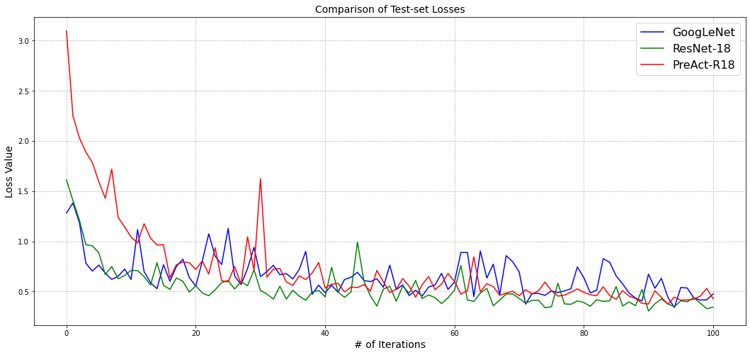
Loss comparison

plt.figure(figsize=(18, 8))

plt.plot(gnet_logs['vl'][:101], color='blue', label='GoogLeNet')

plt.plot(resnet_logs['vl'][:101], color='green', label='ResNet-18')

plt.plot(preresnet_logs['vl'][:101], color='red', label='PreAct-R18')


plt.xlabel("# of Iterations", fontsize=14)
plt.ylabel("Loss Value", fontsize=14)
plt.grid(ls='--', c='grey', alpha=0.5)
plt.title("Comparison of Test-set Losses", fontsize=14)
plt.legend(fontsize=16)
plt.show()

png

Accuracy comparison

plt.figure(figsize=(18, 8))

plt.plot(gnet_logs['va'][:101], color='blue', label='GoogLeNet')

plt.plot(resnet_logs['va'][:101], color='green', label='ResNet-18')

plt.plot(preresnet_logs['va'][:101], color='red', label='PreAct-R18')


plt.xlabel("# of Iterations", fontsize=14)
plt.ylabel("Accuracy", fontsize=14)
plt.grid(ls='--', c='grey', alpha=0.5)
plt.title("Comparison of Test-set Accuracies", fontsize=14)
plt.legend(fontsize=16)
plt.show()

png

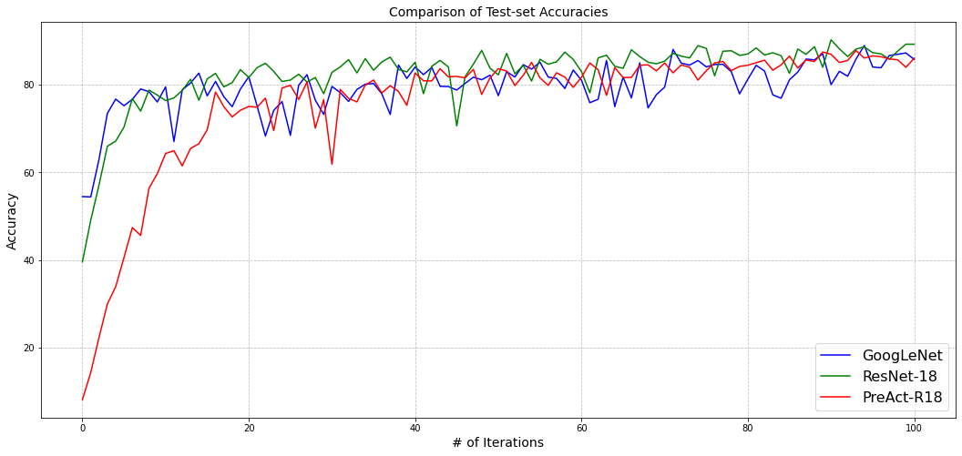
Both the test-set losses and accuracies seems to be converging for all the models. Even though the actual values themselves seems a changing a lot, however, it could be agreed upon that overall the models are still getting improved the best loss and accuracy values are still improving.

All 3 models are observed to perform very similar to each other. On one hand, GoogLeNet falls a little short in terms as it performs worse than both RestNet-18 and PreAct-R18. Among the rest two, its a close match - ResNet-18 dominates PreAct-R18 overs some iterations whereas the opposite is observed in some other iterations.

get_predictions - Function to generate predictions from a data iterator. Since the model outputs class probabilities, the class predictions can be obtained by considering the index with highest probability.

def get_predictions(model, iterator, device):

    model.eval()

    images = []
    labels = []
    probs = []

    with torch.no_grad():

        for (x, y) in iterator:

            x = x.to(device)

            y_pred = model(x)

            y_prob = F.softmax(y_pred, dim=-1)

            images.append(x.cpu())
            labels.append(y.cpu())
            probs.append(y_prob.cpu())

    images = torch.cat(images, dim=0)
    labels = torch.cat(labels, dim=0)
    probs = torch.cat(probs, dim=0)

    return images, labels, probs

Generating predictions

images, g_net_labels, g_net_probs = get_predictions(g_net, testloader, device)
g_net_pred_labels = torch.argmax(g_net_probs, 1)

images, resnet_labels, resnet_probs = get_predictions(res_net, testloader, device)
resnet_pred_labels = torch.argmax(resnet_probs, 1)

images, preresnet_labels, preresnet_probs = get_predictions(preres_net, testloader, device)
preresnet_pred_labels = torch.argmax(preresnet_probs, 1)

Confusion Matrix

One ways of assessing model performance is to evaluate the statistics of correctness of its predictions. Confusion matrix allows us to visualize the confidence of model predictions.

def plot_confusion_matrix(labels, pred_labels, classes, title=None):

    fig = plt.figure(figsize=(10, 10))
    ax = fig.add_subplot(1, 1, 1)
    cm = confusion_matrix(labels, pred_labels)
    cm = ConfusionMatrixDisplay(cm, display_labels=classes)
    cm.plot(values_format='d', cmap='magma_r', ax=ax)
    plt.xticks(rotation=20)
    plt.title(title)
    plt.show()
    
plot_confusion_matrix(g_net_labels, g_net_pred_labels, classes, title="GoogLeNet performance")
plot_confusion_matrix(resnet_labels, resnet_pred_labels, classes, title="ResNet-18 performance")
plot_confusion_matrix(preresnet_labels, preresnet_pred_labels, classes, title="PreAct-R18 performance")

png

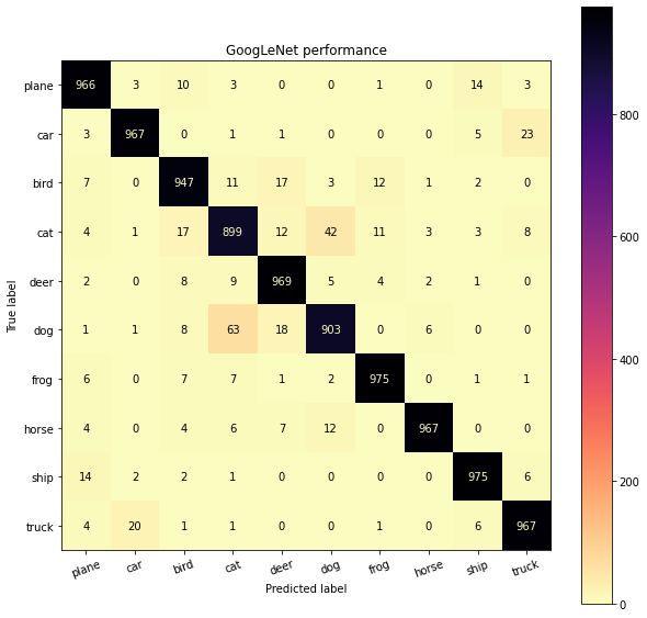
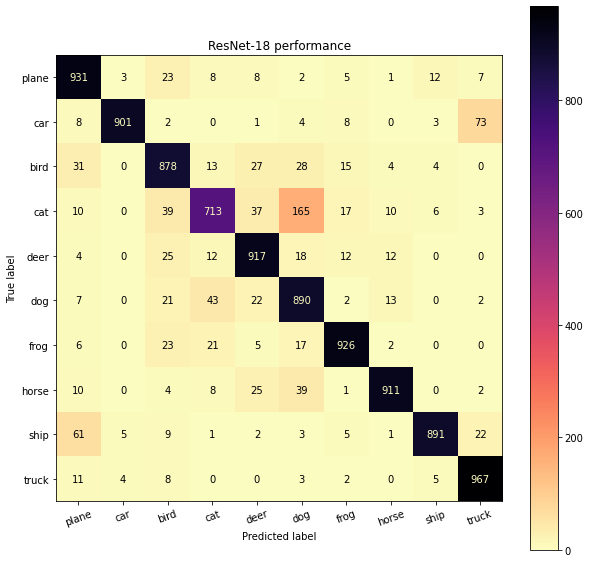
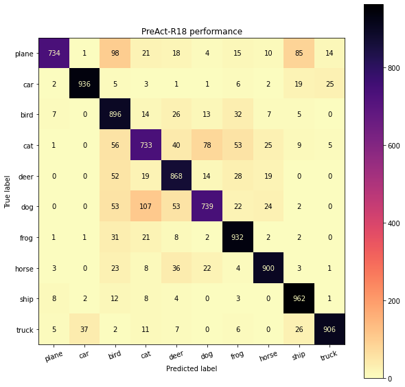
From the confusion matrix, models seem to get mixed up the most between cats and dogs. Another such case is automobile and trucks which is agreeable as trucks and automobiles have bery similar features. One more example is planes and birds, which also from semantics perspective can become hard to recognize due to similar visual features and action of flying.

Discussion

One interesting thing of observation from confusion matrices was that, GoogLeNet (trained for 200 epochs) outperforms both ResNet-18 and PreAct-R18 (both trained for 101 epochs). This wasn’t the case when we performed the training analysis (100 epochs) since the later models are more advanced. What this suggests is that both ResNet-18 and PreAact-R18 have more potential to get trained further and outperform the GoogLeNet, however due to limited time constraints I couldn’t train them further.

The modification to ResNet-18 in the model PreAct-R18, certainly brings some performance gains (observe accuracies for cats, ship etc) where the ResNet-18 model seemed to be least performing. While the modification improves where ResNet-18 performs the poorest (cats), it lacks in some other classes (like dogs) where a drop in performance is observed. Going through the original paper of PreAct-R18 (Identity Mappings in Deep Residual Networks), the authors utilize a depth of 1000 layers to demonstrate the performance gains. It could be that going further deeper, PreAct-R18 should widen the performance gap when trained for more iterations. However, for more shallower networks (~18-22 layers) my observations suggest all the above methods performs very similar and not a significant performance gains are observed

References

[1] Szegedy, Christian, et al. "Going deeper with convolutions." Proceedings of the IEEE conference on computer vision and pattern recognition. 2015.

[2] He, Kaiming, et al. "Deep residual learning for image recognition." Proceedings of the IEEE conference on computer vision and pattern recognition. 2016.

[3] He, Kaiming, et al. "Identity mappings in deep residual networks." European conference on computer vision. Springer, Cham, 2016.

[4] Deep Learning: GoogLeNet Explained - Medium

[5] kuangliu: pytorch-cifar - 2021 Github

Table of Contents:

- 1. Dataset

- 2. Image Recognition Architectures

- 3. Inference and Evaluation

- 4. Discussion

- References

1. CIFAR-10 Dataset

1.1 Data analysis (Abridged)

1.2 Visualization

airplane

automobile

bird

cat

deer

dog

frog

horse

ship

truck

airplane

automobile

bird

cat

deer

dog

frog

horse

ship

truck

2. Image Recognition Architectures

2.1 GoogLeNet

Hyper-parameters:

Testing

Training

2.2 ResNet-18

Hyperparameters

2.3 PreAct-R18 (Identity Mappings in Deep Residual Networks)

Hyper-parameters

3. Inference and Evaluation

3.1 Training Analysis

Loss comparison

Accuracy comparison

Generating predictions

Confusion Matrix

Discussion

References