A Mathematical Persepective and Application on Iris Dataset
In this notebook, I do two things:
- Exploratory data analysis on Iris dataset. I try to show the data-related info, its statistics, and the relationships between features.
- Secondly, I attempt to implement Neural Networks from scratch using NumPy and try to train it on Iris dataset using gradient descent.
Table of Contents:
- 1. Dataset
    1.1 Exploratory Data Analysis .....................
    1.2 Dataset-preprocessing .........................
- 2. Feedforward Neural Networks (using NumPy)
    2.1 Neural Network Training .......................
    2.2 Training Analysis .............................
    2.3 Test Analysis .................................
    2.4 Overfitting ...................................
- 3. Discussion
- References
Reproducibility: This notebook was ran on the following configuration:
- Python version used is 3.7
- All the cpu-intensive processing is done over Intel Xeon(R) chipeset.
import math
import time
import numpy as np
import pandas as pd
import seaborn as sns
import matplotlib.pyplot as plt
%matplotlib inline
1. Dataset
Here, I download the Iris dataset which was discussed at focus in very beginning of the class. The dataset is publicly available at UCI repsitory (https://archive.ics.uci.edu/ml/machine-learning-databases/iris/). For this notebook, I’ve already downloaded the data and can be found as ./Iris.csv.
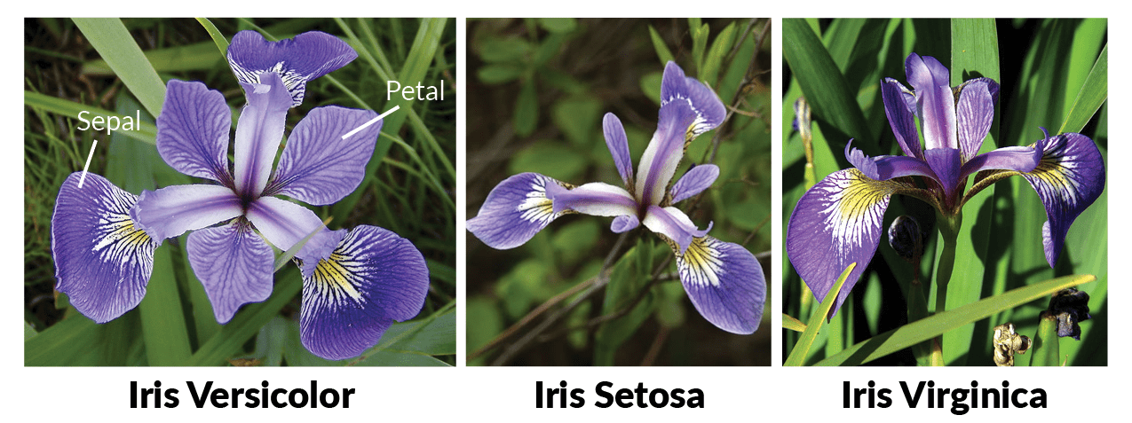
Image Source here
raw_data = pd.read_csv("./Iris.csv")
raw_data.head()
| Id | SepalLengthCm | SepalWidthCm | PetalLengthCm | PetalWidthCm | Species | |
|---|---|---|---|---|---|---|
| 0 | 1 | 5.1 | 3.5 | 1.4 | 0.2 | Iris-setosa |
| 1 | 2 | 4.9 | 3.0 | 1.4 | 0.2 | Iris-setosa |
| 2 | 3 | 4.7 | 3.2 | 1.3 | 0.2 | Iris-setosa |
| 3 | 4 | 4.6 | 3.1 | 1.5 | 0.2 | Iris-setosa |
| 4 | 5 | 5.0 | 3.6 | 1.4 | 0.2 | Iris-setosa |
1.1 Exploratory Data Analysis
I started with understanding what type of data this is. As shown below, the dataset consists of four columns with float64 type values and a fifth column which is an object called Species. As we already know this is a dataset that is widely used to test and understand classification, each data entry could be seen to have 4 features (Sepal length, Sepal Width, Petal Length and Petal Width) based on which it is categorized into species.
raw_data.drop("Id", axis=1, inplace = True)

print("Data technical aspects:")
print(raw_data.info())
Data technical aspects:
<class 'pandas.core.frame.DataFrame'>
RangeIndex: 150 entries, 0 to 149
Data columns (total 5 columns):
 #   Column         Non-Null Count  Dtype
---  ------         --------------  -----
 0   SepalLengthCm  150 non-null    float64
 1   SepalWidthCm   150 non-null    float64
 2   PetalLengthCm  150 non-null    float64
 3   PetalWidthCm   150 non-null    float64
 4   Species        150 non-null    object
dtypes: float64(4), object(1)
memory usage: 6.0+ KB
None
Having a well-balanced distribution among the classes is a very important aspect of machine learning, especially if we are considering to train methods like Neural Networks. They tend to generate unnecessary biasses and inconsistent performance if we have a dataset with unevenly distributed classes. Here, we can see that our data consists of three classes with equally distributed samples among them.
print("Class Distribution:")
print(raw_data["Species"].value_counts())
Class Distribution:
Iris-versicolor    50
Iris-virginica     50
Iris-setosa        50
Name: Species, dtype: int64
Since all the features are real-world measurements of Sepal and Petal in centimeters, they all seem to be roughly on the same scale as can be seen below. Relative smaller values of mean and standard deviation means that feature standardization may not be necessary.
print("Dataset Statistics:")
raw_data.describe()
Dataset Statistics:
| SepalLengthCm | SepalWidthCm | PetalLengthCm | PetalWidthCm | |
|---|---|---|---|---|
| count | 150.000000 | 150.000000 | 150.000000 | 150.000000 |
| mean | 5.843333 | 3.054000 | 3.758667 | 1.198667 |
| std | 0.828066 | 0.433594 | 1.764420 | 0.763161 |
| min | 4.300000 | 2.000000 | 1.000000 | 0.100000 |
| 25% | 5.100000 | 2.800000 | 1.600000 | 0.300000 |
| 50% | 5.800000 | 3.000000 | 4.350000 | 1.300000 |
| 75% | 6.400000 | 3.300000 | 5.100000 | 1.800000 |
| max | 7.900000 | 4.400000 | 6.900000 | 2.500000 |
Data Visualization:
In the following section, I visualize the dataset-related statistics to understand it better. For each feature, I generate violen-plots for all three classes, which helps understand the scale and distribution of each of the features among the different classes.
plt.figure(figsize=(15,10))
plt.subplot(2,2,1)
sns.violinplot(x='Species', y = 'SepalLengthCm', data=raw_data)
plt.subplot(2,2,2)
sns.violinplot(x='Species', y = 'SepalWidthCm', data=raw_data)

plt.subplot(2,2,3)
sns.violinplot(x='Species', y = 'PetalLengthCm', data=raw_data)
plt.subplot(2,2,4)
sns.violinplot(x='Species', y = 'PetalWidthCm', data=raw_data)
plt.show()
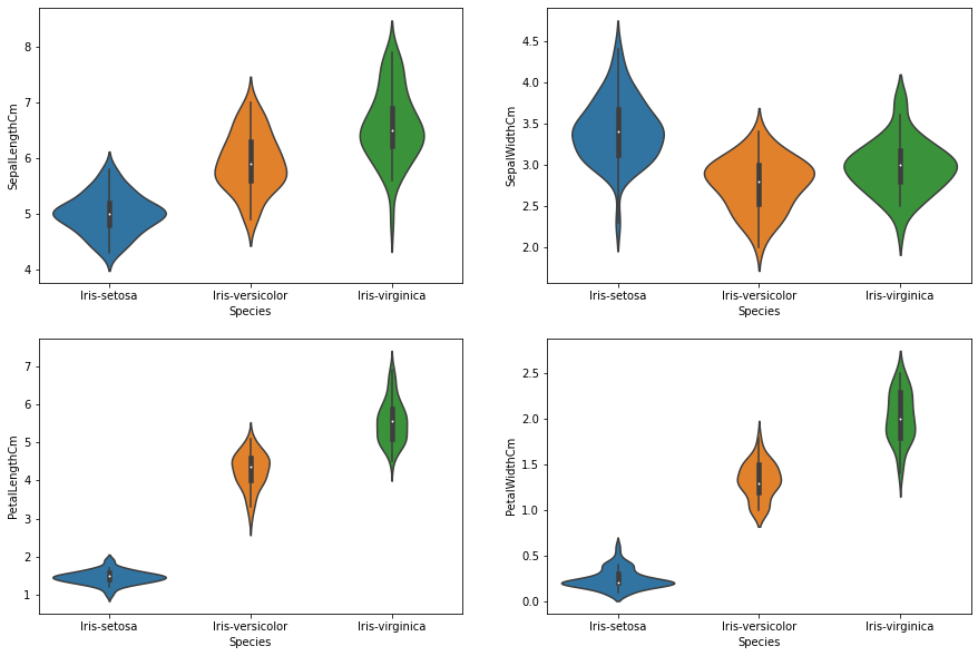
Observations:
- All three species have quite similar Sepal Width values indicating this alone will not be a good distinguishing feature.
- Shorter range of values are observed of Sepal Length for Iris-setosa (4-6 cm) when compared to Iris-virginica which has length ranging from 4 to 8cm.
- All the classes differ widely when their Petal Width are compared essetially making them more seperable.
Here I generate Multivariate plots to better understand the relationships between features:
sns.pairplot(raw_data, hue="Species")
plt.show()
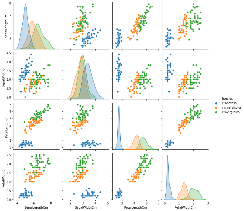
Observations:
- Iris-setosa is observed to be easily identified (blue) and can be easily seperated. On the other hand, Iris-virginica and Iris-versicolor are seen to have quite overlap.
- Petal Length and Petal Width are observed to be the best features to identify various flower types as their feature space is observed to have less overlap, which means they are more seperable.
1.2 Dataset-preprocessing:
The next step would be to process the raw data to a format which can be used to train our classification model.
from sklearn.preprocessing import OneHotEncoder
from sklearn.model_selection import train_test_split
np.random.seed(5720)
Since the features are all float-values at around same scale, we don’t have to change its type. However, the labels (Species) are in text-format which can’t be directly utilized for training our model. Here, I encode the labels using one-hot encoding which will encode each species’ class as a vector consisting of float-values. The result can be seen below:
data_array = raw_data.values

X_features = data_array[:, 0:4]
Y_labels = data_array[:, 4]

one_hot = OneHotEncoder()
Y_transformed = one_hot.fit_transform(Y_labels.reshape(-1,1))
Y_onehot = Y_transformed.toarray()
print("Converted Labels to One-hot encoding:\n")
for i in range(1,150,50):
    print(f"{Y_labels[i]} -> {Y_onehot[i]}")
Converted Labels to One-hot encoding:

Iris-setosa -> [1. 0. 0.]
Iris-versicolor -> [0. 1. 0.]
Iris-virginica -> [0. 0. 1.]
Generalization or in other words, performance of models on unseen data is very crucial in machine learning. Therefore, I try to create train-test sets from dataset. Train-set will be used for training our model and Test-set can be used to evaluate our model performance on unseen data. Here, I will split the dataset into these two sets, 80% (train-set) of which we will use to train our models and 20% (test-set) that we will hold back as a test dataset.
test_size = 0.20

def process_data(X, Y):
    X, Y = X[:, :, np.newaxis], Y[:, :, np.newaxis]
    X_train, X_test, Y_train, Y_test = train_test_split(X, Y, test_size=test_size)

    X_train, X_test = X_train.astype(float), X_test.astype(float)
    Y_train, Y_test = Y_train.astype(float), Y_test.astype(float)

    train = [(X_train[i], Y_train[i]) for i in range(len(X_train))]
    test = [(X_test[i], Y_test[i]) for i in range(len(X_test))]

    return train, test

train, test = process_data(X=X_features, Y=Y_onehot)
input_dimensions, output_dimensions = len(train[0][0]), len(train[0][1])
print('Number of Input Features: ', input_dimensions)
print('Number of Output classes: ', output_dimensions)
Number of Input Features:  4
Number of Output classes:  3
2. Feedforward Neural Networks (using NumPy)
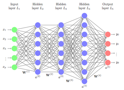
Image source here
In this section, I implement a class representing a general feed-forward neural network from scratch that utilizes the sigmoid activation function. Additionally, I have constructed gradient descent mechanism to train my implemented neural network. The class also consists of several helped-functions such as generating training logs, evaluating the predictions etc.
Below, I give mathematical intuition behind each of the functions (highlighted in brackets) that is present in my implementation of feedforward neural network.
Let’s start with the error:
\(error = \frac{1}{2} (yPred-Y)^2\)
- Here, \(yPred\) =
forward_Prop\((X)$, and\)Y$$ is the desired output value from the neural network.
- The feedforward operation (
forward_Prop) is a fairly simple process that consists of successive matrix-vector multiplications. For a single neuron with index \(i\) in layer \((l+1)\), this process can be formulated as follows:
where \(w_{ij}^{l}\) is the weight of the neuron, \(a_j^{(l)}\) is the input that particular neuron is receiving and \(b_i^{(l+1)}\) is the bias that will be added to output of the \(i^{th}\) neuron.
- Once we have initialized all the weights \(W\), we need to iteratively update it such that cost \(J\) is minimized.
- Consider layer \(L\), Computing \(\frac{\partial}{\partial W^{(L)}}(Cost \;J)\)
\(\frac{\partial}{\partial W^{(L)}}(Cost\; J) = Cost \;J' \times \frac{\partial}{\partial W^{(L)}}(yPred)\)
- where \(CostJ'\) is the derivative of the Cost function (
grad_cost)
- Let’s compute \(\frac{\partial \;yPred}{\partial W^{(L)}}\)
- We use Sigmoid activation function, so \(yPred\) can be written as:
\(yPred = Sigmoid(X^{(L)}*W^{(L)}+b^{L})\)
- So,
\(\frac{\partial\;yPred}{\partial W^{(L)}} = \frac{\partial}{\partial W^{(L)}}\left(Sigmoid\left(X^{(L)}.*W^{(L)}+b^{L})\right)\right) = Sigmoid^{'}\left(X^{(L)}.*W^{(L)}+b^{L})\right)*\left(\frac{\partial}{\partial W^{(L)}}\left((X^{(L)}.*W^{(L)}+b^{L})\right)\right)\)
- Here \(Sigmoid'\) is the derivative of the Sigmoid activation function (
g_prime).
- Computing \(\frac{\partial}{\partial W^{(L)}}((X^{(L)}.*W^{(L)}+b^{L}))\)
- It can be seen that \(\frac{\partial }{\partial W^{(L)}}((X^{(L)}.*W^{(L)}+b^{L})) = X^{(L)}\), where \(X^{L}=Sigmoid(W^{L-1}*X^{L-1}+b^{L-1})\)
- Computing gradients in backward propogation (back_prop)
-
Consider a variable \({\Delta}W^{(L)}\), such that: \({\Delta}W^{(L)} = Cost'J \times Sigmoid' (W^{(L)}\times X^{(L)}+b^{L})\)
-
For each iteration (\(i\)) starting from the second last layer to the first: \({\Delta}b^{(i)} = {\Delta}W^{(L)}\;\; \text{(Derivative w.r.t}\;\; \partial b^{L}\; \text{is just}\; \Delta W^{(L)}\)
\({\Delta}W^{(i)} = {\Delta}W^{(L)} * X^{L} \;\;\; \text{(where,}\; X^{L}=Sigmoid(W^{i-1}*X^{i-1}+b^{i-1})\) \({\Delta}W^{(L)} = {(\Delta}W^{(L)} * W^{i}) * Sigmoid'(W^{i}*X^{i}+b^{i})\)
- Updating the parameters (SGD_step)
\(W^{(i)} \leftarrow W^{(i)} + \eta*{\Delta}W^{(i)}\) \(b^{i} \leftarrow b^{i} + \eta*{\Delta}b^{i}\)
class Network:
    def __init__(self, sizes):
        """
        Feedforward Neural Network

        sizes: list [input_dimensions, hidden_layer_dimensions, output_dimensions]
        L: length of the layer
        biases: list containing biases values for each layer
        weights: list containing weights for each layer

        Parameters:
        sizes: list containing dimenions of the neual network
        """
        self.L = len(sizes)
        self.sizes = sizes
        self.biases = [np.random.randn(n, 1) for n in self.sizes[1:]]
        self.weights = [np.random.randn(n, m) for (
            m, n) in zip(self.sizes[:-1], self.sizes[1:])]

        self.acc_train_array = []
        self.acc_test_array = []

    def sigmoid(self, z, threshold=20):
        """
        Sigmoid activation function
        """
        z = np.clip(z, -threshold, threshold)
        return 1.0 / (1.0 + np.exp(-z))

    def g_prime(self, z):
        """
        Derivative of sigmoid activation function
        """
        return self.sigmoid(z) * (1.0 - self.sigmoid(z))

    def forward_prop(self, a):
        """
        Forward propagation:
        : Do layerwise dot product between the input and the weights,
        : adding the coresponding biases and taking activations of it
        : starting from the first layer then forward and return the final output.
        """
        for (W, b) in zip(self.weights, self.biases):
            a = self.sigmoid(np.dot(W, a) + b)
        return a

    def cost(self, yhat, y):
        """
        Cost Function
        : Cost(a,y) = (yhat-y)^2/2
        """
        return 0.5*np.square(a-y)

    def grad_cost(self, yhat, y):
        """
        Gradient of cost function:
        : Derivative of Cost(yhat,y)
        """
        return (yhat - y)

    def log_train_progress(self, train, test, epoch):
        """ Logs training progres.
        """
        acc_train = self.evaluate(train)
        self.acc_train_array.append(acc_train)
        if test is not None:
            acc_test = self.evaluate(test)
            self.acc_test_array.append(acc_test)
            print("Epoch {:4d}: Train acc {:10.5f}, Test acc {:10.5f}".format(epoch+1, acc_train, acc_test))
        else:
            print("Epoch {:4d}: Train acc {:10.5f}".format(epoch+1, acc_train))

    def back_prop(self, x, y):
        """
        Back propagation for computing the gradients

        : Once forward prop completes (implemented inside), initate list of gradients (dws, dbs),
        : where each element of list stores the corresponding gradients of that layer.
        : For each layer compute the gradients and update the list (dws, dbs) and return it.
        Parameters:
            x: Sample features
            y: Sample labels

        RETURN: (dws, dbs)
                 dws: list of layerwise derivative of weights
                 dbs: list of layerwise derivative of biases
        """
        a = x
        # List initialized for storing layer-wise output before it is fed to activations
        pre_activations = [np.zeros(a.shape)]
        # List initialized for storing layer-wise activations
        activations = [a]

        # Forward propogation to compute layer-wise pre_activations and activations
        for W, b in zip(self.weights, self.biases):
            z = np.dot(W, a) + b
            pre_activations.append(z)
            a = self.sigmoid(z)
            activations.append(a)

        db_list = [np.zeros(b.shape) for b in self.biases]
        dW_list = [np.zeros(W.shape) for W in self.weights]

        delta = self.grad_cost(activations[self.L-1], y) * \
            self.g_prime(pre_activations[self.L-1])

        for ell in range(self.L-2, -1, -1):
            db_list[ell] = delta
            dW_list[ell] = np.dot(delta, activations[ell].T)
            delta = np.dot(self.weights[ell].T, delta) * self.g_prime(pre_activations[ell])
        return (dW_list, db_list)

    def SGD_step(self, x, y, eta):
        """
        Update the values of weights (self.weights) & biases (self.biases)
        : Get values of gradients (dws, dbs) by calling back_prop
        : and update parameters using obtained gradients & learning rate eta

        Parameters:
            x: single sample features.
            y: single sample target.
            eta: learning rate.
            lam: Regularization parameter.

        RETURN: none
        """
        dWs, dbs = self.back_prop(x, y)
        self.weights = [W - eta * (dW) for (W, dW) in zip(self.weights, dWs)]
        self.biases = [b - eta * (db) for (b, db) in zip(self.biases, dbs)]

    def train(self, train, epochs, eta, verbose=True, test=None):
        """
        Training routine for the neural network. For each epoch the following is done:
        : shuffle the training dataset.
        : call self.SGD_step which will in turn call backprop & update parameters
        : Call self.log_train_progress according to the verbose

        Paramerers:
            train: Training set -> list containing tuple (Training Feature, Training label)
            epochs: Number of epocs to run
            eta: Learning rate
            verbose: True to print accuracy updates, False otherwise
            test: Test set -> list containing tuple (Test Feature, Test label)
        """
        n_train = len(train)
        for epoch in range(epochs):
            perm = np.random.permutation(n_train)
            for kk in range(n_train):
                self.SGD_step(*train[perm[kk]], eta)
            if verbose and epoch == 0 or (epoch + 1) % 20 == 0:
                self.log_train_progress(train, test, epoch)

    def predict(self, data):
        """
        Generate predictions
        : Calls forward propagation to generate predictions

        Parameters: data: (X,Y)

        RETURN: yhat (predictions)
        """
        preds = []
        for x, y in data:
            yhat = self.forward_prop(x)
            preds.append(yhat)
        return preds

    def evaluate(self, test):
        """
        Evaluate current model
        : computes the fraction of labels matching
        test : (test_x, test_y)
        """
        ctr = 0
        for x, y in test:
            yhat = self.forward_prop(x)
            ctr += yhat.argmax() == y.argmax()
        return float(ctr) / float(len(test))
2.1 Neural Network Training
It’s time to train the above implemented neural network. Generally, The hidden layer dimension (no. of neurons) is seen to affect the classification capabilities of a neural network. Here I try training my neural network with three configurations- each consisting of different hidden layer width (5, 20 and 50). I train each of these configuations for 100 epochs with a learning rate of \(1e-2\). For every 20 epochs, I report both the train and the test performances.
nns = []
for hidden_layer_dimensions in [5, 20, 50]:
    print('\nHidden Layer Dimensions: ', hidden_layer_dimensions)
    nn = Network([input_dimensions, hidden_layer_dimensions, output_dimensions])
    nn.train(train, epochs=100, eta=0.2, verbose=True, test=test)
    nns.append(nn)
Hidden Layer Dimensions:  5
Epoch    1: Train acc    0.56667, Test acc    0.70000
Epoch   20: Train acc    0.94167, Test acc    1.00000
Epoch   40: Train acc    0.92500, Test acc    0.96667
Epoch   60: Train acc    0.98333, Test acc    0.96667
Epoch   80: Train acc    0.98333, Test acc    0.96667
Epoch  100: Train acc    0.95000, Test acc    0.96667

Hidden Layer Dimensions:  20
Epoch    1: Train acc    0.31667, Test acc    0.40000
Epoch   20: Train acc    0.96667, Test acc    1.00000
Epoch   40: Train acc    0.97500, Test acc    1.00000
Epoch   60: Train acc    0.97500, Test acc    1.00000
Epoch   80: Train acc    0.95833, Test acc    0.96667
Epoch  100: Train acc    0.97500, Test acc    1.00000

Hidden Layer Dimensions:  50
Epoch    1: Train acc    0.65833, Test acc    0.70000
Epoch   20: Train acc    0.80833, Test acc    0.83333
Epoch   40: Train acc    0.97500, Test acc    0.96667
Epoch   60: Train acc    0.98333, Test acc    0.93333
Epoch   80: Train acc    0.97500, Test acc    0.93333
Epoch  100: Train acc    0.97500, Test acc    1.00000
2.2 Training Analysis
Here, I plot the the evolution of training accuracy as the epochs are incremented for all three configuations.
fig, ax = plt.subplots(nrows=1, ncols=1, figsize=(15,7))
epochs_array = [i for i in range(1, 120, 20)]

ax.plot(epochs_array, nns[0].acc_train_array, color="blue", ls='dashed',  label="5")
ax.plot(epochs_array, nns[1].acc_train_array, color="green", ls='dashed',  label="10")
ax.plot(epochs_array, nns[2].acc_train_array, color="red", ls='dashed', label="50")

ax.legend(title='Hidden layer\n   neurons', loc="lower right", fontsize=16)
plt.rcParams['legend.title_fontsize'] = 'xx-large'
ax.set_xlabel("epochs", fontsize=16)
ax.set_ylabel("Train accuracy", fontsize=16)
plt.title("Train performance over epochs", fontsize=18)
plt.grid(ls='--', color='gray', alpha=0.5)
plt.show()

Observations:
- All three configurations are observed to be converging.
- Hidden layer width of 5 (blue) and 10 (green) are observed to train and reach the optimal faster as compared to network with 50 hidden-layer width (red). This could be explained due to the fact that larger neural networks, having more parameters takes more iterations to get trained.
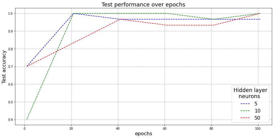
2.3 Test Analysis
Here, I generate a very similar plot with modification of being on the test-set.
fig, ax = plt.subplots(nrows=1, ncols=1, figsize=(15,7))
epochs_array = [i for i in range(1, 120, 20)]

ax.plot(epochs_array, nns[0].acc_test_array, color="blue", ls='--', label="5")
ax.plot(epochs_array, nns[1].acc_test_array, color="green",  ls='--', label="10")
ax.plot(epochs_array, nns[2].acc_test_array, color="red",  ls='--', label="50")

ax.legend(title='Hidden layer\n   neurons', loc="lower right", fontsize=16)
plt.rcParams['legend.title_fontsize'] = 'xx-large'
ax.set_xlabel("epochs", fontsize=16)
ax.set_ylabel("Test accuracy", fontsize=16)
plt.title("Test performance over epochs", fontsize=18)
plt.grid(ls='--', color='gray', alpha=0.8)
plt.show()
Observations:
- Again, all three configurations are observed to have converged and are giving very good test-set performance.
- One interesting thing to note here is that, having a bigger neural network doesn’t necessarily imply getting better performance. As can be observed from above, the width-10 network (green) is observed to surpass a much bigger width-50 network (red) almost always. The reason could be that width-50 model could be overparamterized which means- it has more modelling capability than what is required for the classification task. This suggests that simpler models generally tend to have higher generalizability on unseen set as compared to more complex overparamaterized networks.
- Additionally, width-10 network (green) also beats the width-5 network (blue) over test-set. The fact that width-5 network’s performance not improving over iterations means it has saturated and just doesn’t have enough modelling capability to get optimal results for our classification task. The width-10 network is oberved to be at a balance here.
2.4 Overfitting
Here I train a neural network for a much larger no. of iterations than what is required.
hidden_layer_dimensions = 50
nn2 = Network([input_dimensions, hidden_layer_dimensions, output_dimensions])
nn2.train(train, epochs=400, eta=0.2, verbose=True, test=test)
Epoch    1: Train acc    0.38333, Test acc    0.30000
Epoch   20: Train acc    0.97500, Test acc    0.96667
Epoch   40: Train acc    0.97500, Test acc    1.00000
Epoch   60: Train acc    0.91667, Test acc    0.96667
Epoch   80: Train acc    0.91667, Test acc    0.96667
Epoch  100: Train acc    0.95000, Test acc    0.90000
Epoch  120: Train acc    0.95000, Test acc    0.96667
Epoch  140: Train acc    0.94167, Test acc    0.86667
Epoch  160: Train acc    0.95000, Test acc    0.96667
Epoch  180: Train acc    0.97500, Test acc    1.00000
Epoch  200: Train acc    0.97500, Test acc    1.00000
Epoch  220: Train acc    0.98333, Test acc    0.96667
Epoch  240: Train acc    0.97500, Test acc    1.00000
Epoch  260: Train acc    0.98333, Test acc    0.96667
Epoch  280: Train acc    0.97500, Test acc    1.00000
Epoch  300: Train acc    0.98333, Test acc    0.96667
Epoch  320: Train acc    0.98333, Test acc    0.96667
Epoch  340: Train acc    0.97500, Test acc    0.96667
Epoch  360: Train acc    0.95000, Test acc    0.86667
Epoch  380: Train acc    0.98333, Test acc    0.96667
Epoch  400: Train acc    0.97500, Test acc    0.96667
fig, ax = plt.subplots(nrows=1, ncols=1, figsize=(15,7))
epochs_array = [i for i in range(1, 420, 20)]

ax.plot(epochs_array, nn2.acc_train_array, color="blue", ls='--', label="Train")
ax.plot(epochs_array, nn2.acc_test_array, color="red", ls='--', label="Test")

ax.legend(title='Data', loc="lower right", fontsize=16)
plt.rcParams['legend.title_fontsize'] = 'xx-large'
ax.set_xlabel("epochs", fontsize=16)
ax.set_ylabel("Accuracy", fontsize=16)
plt.title("Performance over epochs (Hidden layer dim: 50)", fontsize=18)
plt.grid(ls='--', color='gray', alpha=0.8)
plt.show()
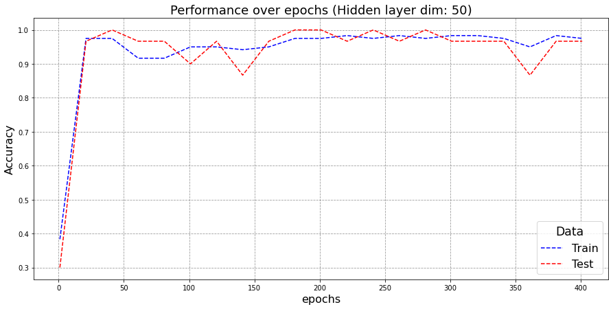
- Training for more iterations doesn’t necessarily imply a greater test-performance. In fact, after 300 epochs, a decrease in test performance is observed even though the train performance is still getting better. This refers to overfitting. Since neural networks are trying to model the train-set and when trained for larger iterations, they tend to learn the train data itself than the underlying distribution which leads to poor performance on unseen test-set.
3. Discussion
From the exploratory analysis of Iris dataset, we observed not all the features have equal seperable characteristics. Here, features of the Petals could help better distinguish the different classes as compared to the attrcibute Sepal. The features of the dataset were relatively on the same scale due to which we may not need to standardize it. Additionally, Iris has a balanced class distribution with each having 50 entries, this is good for making the training of a neural network stable and more consistent.
From the analysis on Neural networks, the first crucial thing to note was that having a bigger network doesn’t necessarily perform better than simpler/smaller networks. The required complexity of a network completely depends on the task at hand. Going with a very small network may lead to underparamaterization which means the network doesn’t have enough capacity to learn the underlying distribution to get optimal results. On the other hand, very large networks requires more training and may also lead to overfitting, which essentially means that network has started to learn the training data itself which leads to poor performance on unseen data. Overfitting also becomes likely when trained for huge no. of iterations as we discussed above.
Generally, we want a model with balanced complexity, which is something that could be derived solely based on hit-trial method. Essentially models with different configurations needs to trained and tested to see what optimal configuration performs better. Additionally, the test-set performance needs to be monitored continuously over the iterations to avoid the case of overfitting. There are other variations or model designs such as Dropouts (dropping neurons randomly during training) that are widely used these days which let’s you train larger networks while reducing the case of overfitting. It’ll be surely intersting to analyze the various perfromances to detect any underlying pattern for different hyperparameters and design choices to get the optimal network.
References
[1] Dua, D. and Graff, C. (2019). UCI Machine Learning Repository [http://archive.ics.uci.edu/ml]. Irvine, CA: University of California, School of Information and Computer Science

[2] Casper Hansen (2019) [https://mlfromscratch.com/neural-networks-explained/]

[3] Maziar Raissi (Github- Applied Deep Learning) - Lecture Notes [https://github.com/maziarraissi/Applied-Deep-Learning]